X-Ray Fluorescence Spectrometry—Theory and Practice

This article is compiled based on the United States Pharmacopeia (USP) – 2025 Edition

Issued and maintained by the United States Pharmacopeial Convention (USP)

DOWNLOAD PDF HERE

1 INTRODUCTION 

This general chapter provides information regarding the theory and acceptable practices for the consistent analysis and interpretation of X-ray fluorescence spectroscopic data. X-ray fluorescence (XRF) spectrometry is an instrumental technique based on the measurement of characteristic X-ray photons caused by the excitation of atomic inner-shell electrons by a primary X-ray source. The XRF technique can be used for both qualitative and quantitative analysis of liquids, powders, and solid materials. Although some vendors supply radioactive isotope-based source instruments, nearly all modern instruments use an X-ray tube as the source. 

2 PRINCIPLES OF X-RAY FLUORESCENCE SPECTROMETRY 

The X-rays produced by an X-ray tube include characteristic lines corresponding to the anode material, and a continuum also known as Bremsstrahlung radiation. Both types of X-rays can be used to excite atoms in a specimen and thus induce X-rays. The intensity of both of these types can be adjusted by the voltage and current settings of the X-ray generator. These parameters can be adjusted to optimize the ux of X-ray photons for each element of interest. Further adjustments, such as the addition of filters in the primary beam, can be used to remove undesirable and potentially interfering tube spectral lines. Secondary targets may be used to produce an excitation X-ray beam that differs from the primary X-ray tube spectrum, with the aim of achieving optimum excitation conditions. Numerous instrument designs with different geometrical configurations, for example, secondary filters and polarization, are used to optimize X-ray detection and reduce background contributions. 

Although many variations exist, XRF instrumentation can be divided into two categories: wavelength-dispersive XRF (WDXRF) and energy dispersive XRF (EDXRF) instruments. The main distinguishing factor between these two technologies is the method used to separate the spectrum emitted by all atoms in the sample according to X-ray photon energy. 

The energy (or the wavelength) of the X-ray photon is characteristic of a given electron transition in an atom, and is therefore qualitative in nature. The intensity of the emitted radiation is indicative of the number of atoms in the sample, and therefore constitutes the quantitative nature of the technique. 

3 PHYSICS OF X-RAY EXCITATION AND EMISSION 

3.1 Ionization and the Photo-Electric Effect 

The emission of characteristic X-ray radiation results from an electron transition between two inner shells of an atom, after ionization. After, for example, the ejection of an electron from the K-shell, the atom is ionized and the ion is left in a high-energy state, E₁ , with E₁ being equal to the energy required to remove the K-electron from the shell to a situation where it is at rest (no remaining kinetic energy) at infinite distance from the nucleus. This interaction between electromagnetic radiation (a photon) and an atom resulting in an electron being excited is called the photo-electric effect. It is typically the largest contribution to absorption of X-rays. E₁ thus corresponds to the binding energy of the electron, which is identical to the energy of the atomic level. The excited state has a very limited life span, and will decay rapidly by a transition of an electron from an outer shell to the vacancy in the inner shell. The atom is still ionized, with an electron vacancy in the other shell. Let the energy state after this transition be represented by E₂, corresponding to the binding energy of the electron prior to the transition. The energy difference, ΔE, is represented by 

ΔE = E₁ − E₂ [1] 

and can be released in two competing processes: the Auger effect, or the emission of a photon. For XRF, obviously the latter is of interest. The energy of the photon emitted is thus equal to ΔE. The binding energies of the inner electrons are not affected by the chemical state of the atom concerned. The atomic energy levels are unique (characteristic) to the element, thus the energy difference between two given levels is also a characteristic. Therefore, the resulting X-ray photon is called a characteristic photon. The energy of the characteristic photons is varying in a systematic way with the atomic number Z of the elements, a fact that can be represented using Moseley's law [1]: 

E_photon = k(Z − s)²[2] 

where k is a constant for a given series (as defined by the shell with the initial electron vacancy) and s is the screening constant. A fairly complete tabulation of the energies of characteristic radiation can be found in the work by Bearden [2]. Assume that the initial vacancy was created in the K-shell. After an electron transition from, for example, the L3-shell, the atom still has an electron vacancy, but in the L3-shell, while a photon with an energy E corresponding to 

E_photon = E_k − E_L3 [3] 

has escaped the atom. The vacancy in the L3-shell can subsequently be filled by an electron from the M5-shell (assuming that this is a high atomic-number element). This results in a vacancy in the M5-shell that can then decay further. At the end of this cascade, the ion is back in the neutral state. 

3.2 Scattering 

The most important interaction between X-rays and matter is the photo-electric effect, described above. Two other mechanisms are coherent and incoherent scatter. 

3.2.1 Coherent scatter 

Coherent scatter is elastic scattering of electromagnetic radiation by a free, charged particle. It is also known as Thomson scattering. The electric eld of the incident photon accelerates the charged particle. This particle will subsequently emit radiation with the same energy as the incident photon, but travelling in a different direction. 

3.2.2 Incoherent scatter 

Incoherent scatter of a photon is usually called Compton scatter. Compton scatter is inelastic in nature. Both momentum and energy are conserved in the process. After Compton scattering, the electron has acquired considerable momentum (and is excited from the atom), and a photon with a longer wavelength than the incident photon is emitted (see Figure 1). The conservation of energy and of momentum leads to a simple relationship between the scattering angle Φ and the wavelength difference Δλ between the incident and the Compton scattered photon: 

Δλ = 0.00243 ·  (1 − cosΦ) [4] 

Equation [4] calculates the wavelength shift in nm. The peaks of Compton scattered radiation are typically broader than those corresponding to characteristic radiation or coherently scattered radiation. The reason is that most X-ray fluorescence spectrometers do not have a collimated incident beam. The incident angle on the specimen can thus vary significantly. This contributes to wide variation in total scattering angles Φ, leading to variation in Δλ. 

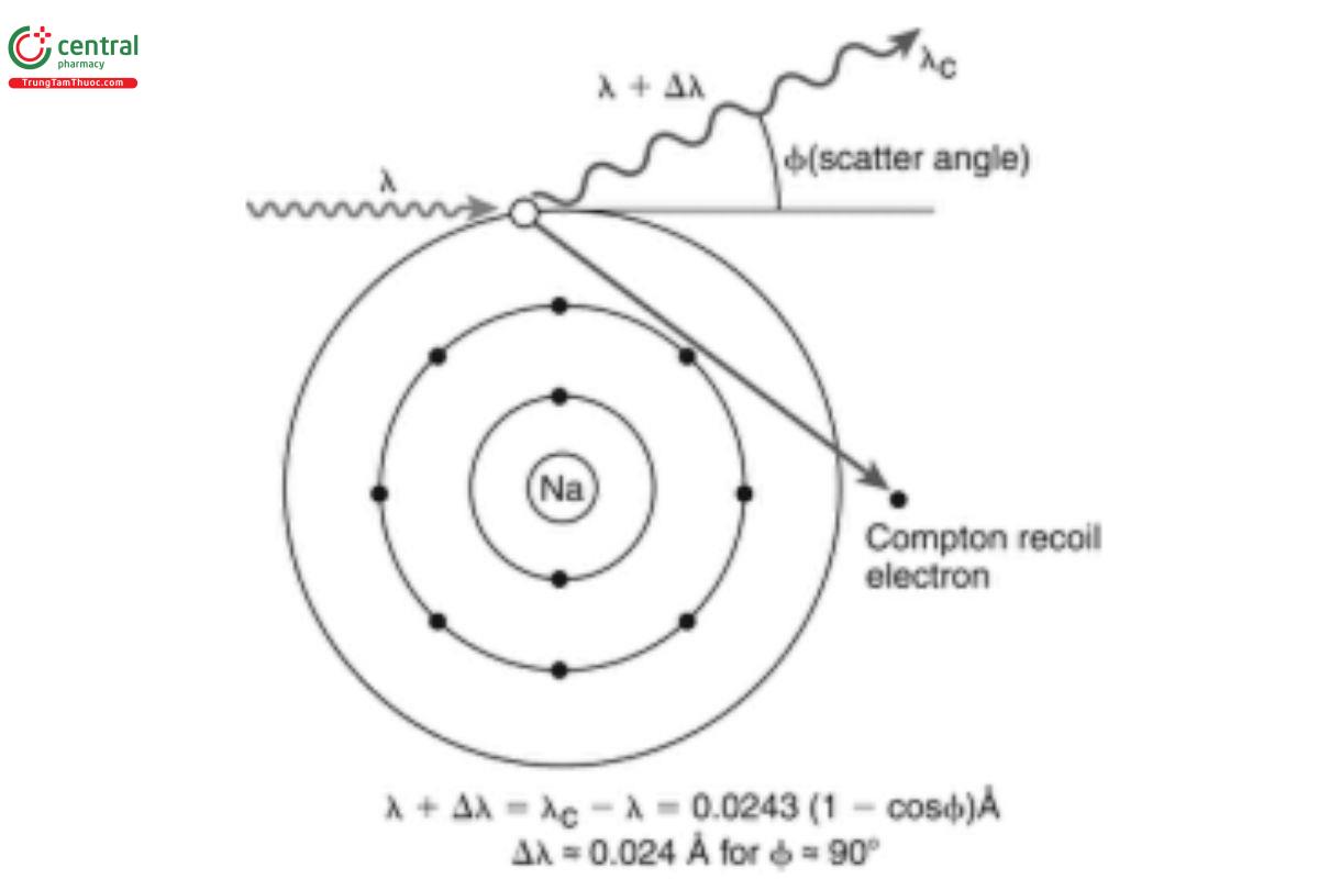
Figure 1. Compton scattering of an X-ray photon; Φ is the scattering angle (from Willis and Duncan [3] with permission). 3.3 Conversion between Energy and Wavelength 

Photons exhibit a wave-particle duality [4]. The energy, E, of the “particle” and the wavelength λ of the “wave” are related through Planck's constant, h: 

E =hc/λ  [5] 

where E is the photon energy; h is Planck's constant; and c is the speed of light in vacuum. By substituting these values in Equation [5], and expressing photon energy E in keV and wavelength λ in nm, the following is obtained: 

E =1.24 / λ [6] 

This allows quick and easy conversion between energy and wavelength scales. Note that shorter wavelengths correspond to higher energies. 

Commonly, textbooks designed around WDXRF will use wavelength units for the characteristic radiation. On the other hand, when dealing with EDXRF, the scale of choice is an energy scale with keV as the unit. Photon energy can be converted to photon wavelength and vice versa using Equation [6]. The frequency of the electromagnetic radiation (which can be calculated using c/λ or from E/h) is not used when relating to XRF analysis. 

3.3 The Electromagnetic Spectrum 

The X-ray range is typically the spectral range between 0.01 and 10 nm, and it spans 4 orders of magnitude. In practice, however, the range of X-rays commonly analyzed varies from about 0.04 to 1 nm. 

The X-ray region of the electromagnetic spectrum can also be expressed in terms of the characteristic radiation of the elements. Most wavelength-dispersive X-ray spectrometers can be equipped to analyze characteristic lines between about 0.04 and 4.4 nm. This allows analysis of all elements in the periodic table from carbon upwards (Z = 6). With dedicated analyzers, the elemental range can be extended to include beryllium, although issues with limited specificity and sensitivity severely limit the practical applications for the quantitative analysis of beryllium. 

3.4 Selection Rules 

The transitions in the process described above are governed by quantum-mechanical selection rules. XRF radiation is observed with reasonable probability only from those transitions where 

Δj = –1, 0, +1      and         Δl = –1 or +1 

where j and l are the usual quantum numbers. The correspondence between shell designations (K, L, M…) and the quantum numbers n, l, and m is given in Table 1. This means that in transitions such as K ← L1 and L1 ← M1, both shells with l = 0 for initial and nal state are forbidden radiative transitions. These transitions, however, can be accompanied by the emission of an Auger electron. 

Table 1. Correspondence between Shell Designations (K, L, M, N) and Quantum Numbers (n, l, m) 

After the initial vacancy has been created, the ion is in a highly excited state. After an electron transition, for example, K ← L3, an energy equal to the difference in the binding energies (see Equation [3]) between the two shells involved can be released. In the case on hand, this gives rise to the emission of a Kα photon. Photon emission is, however, only one of two competing processes. The other is the emission of an Auger electron. This is the process in which the energy is transferred to another electron, which escapes the ion with a certain kinetic energy E_Kin . The kinetic energy can be calculated in much the same fashion as the photon energy, using the energy levels from the shells Kin involved. If the energy released from the K ← L3 transition is transferred to an L1 electron, the kinetic energy can be calculated from 

E_Kin = E_Auger = E_K − E_L1 − E_L3 [7] 

The kinetic energy of the Auger electron is characteristic because it is made up of characteristic quantities. The vacancies created after the emission of an Auger electron can subsequently decay, either by other Auger electrons or by photons. 

3.5 Fluorescence Yield 

The fluorescence yield (symbol ω) is defined as the probability that a vacancy is filled through a radiative transition. For the K-shell this is simply 

ωK =   lK / nK [8] 

where I_K is the total number of K-shell X-ray photons and n is the number of vacancies created in the K-shell. For the L-shell and M-shell, a similar definition applies for each of the subshells, but the number of primary vacancies needs to be corrected for the cascade effects and the occurrence of Coster-Kronig transitions [5]. These are nonradiative transitions between subshells having the same principal quantum number. Data regarding values for fluorescence yields can be found in the work by Bambynek et al. [5] and Hubbell et al. [6]. 

3.6 Counting Statistical Error 

The counting statistical error (CSE) is the uncertainty in the measurement of the number of photons, which is subject to a Poisson distribution. The distribution of the number of photons can be approximated by a normal distribution, because the number of photons counted is usually  sufficiently large. The standard deviation σ_N of an intensity measurement of N counts is given by the square root of the N number of counts: 

σ_N =    √N  [9] 

Most measurements in XRF are now expressed as an intensity, I, which is simply the ratio of the number of photons counted divided by the measuring time, t. The counting statistical error on a measured intensity can be calculated using 

σ = √(l/t)  [10] 

This indicates that the counting statistical error on an intensity measurement becomes smaller with longer measurement times. Measuring longer on an XRF instrument (under otherwise constant conditions of measurement) reduces the relative uncertainty on the measurement. This is generally applicable until the resulting CSE becomes comparable to the overall instrument error. For high-end instrumentation, the order of magnitude of this overall instrument error is about 0.1% or better. Performing measurements with a CSE significantly lower than the overall instrumental error will not lead to more precise results. The CSE thus imposes a theoretical lower limit to the precision of an X-ray measurement. The contribution of the instrumental errors is added to the CSE to obtain the total error on the measurement. 

The intensity of a photon beam is calculated from the number of photons collected divided by the time taken for the measurement, expressed in counts per second (cps) or kilocounts per second (kcps). 

3.7 Detection Limit 

The lower limit of detection (LLD) is defined as the concentration that will yield a positive intensity above background intensity with a given confidence level. For analysis near the detection limit, the intensity of the peak will be comparable to the intensity of the background. For example, a net signal that is 3 times larger than the CSE of the background will satisfy this criterion with 99.7% confidence. This intensity can then be converted to a concentration using the sensitivity, S, of the spectrometer for the analyte considered: 

LLD =   (k ×  CSE) / S  [11] 

where k is a factor depending upon the confidence level chosen, S is the sensitivity (expressed as net intensity per unit concentration), and CSE is the counting statistical error of the determination. Substituting Equation [10] where σ_I is the CSE of the intensity of the background yields 

LLD =   k/S. √ (l_B/t)  [12] 

where I_B is the intensity of the background radiation at the analytical line considered. The LLD can be improved by the following: B 

• Increasing the sensitivity, S, of the spectrometer 
• Decreasing the intensity of the background, I_B 
•  Increasing the measurement time, t. 

The third method, increasing the measurement time, seems to be an especially easy way to improve detection limits, but it is limited because long counting times can make the method impractical. Hence, for a given spectrometer configuration, any increase in the sensitivity results in a similar increase of the background intensity. Quadrupling the sensitivity also leads to a 4-fold higher background intensity and an improvement of the LLD by a factor of 2. 

3.8 Nomenclature of X-Ray Emission Lines 

There are different nomenclatures in use involving the designation of the X-ray emission lines. The International Union of Pure and Applied Chemistry (IUPAC) published a systematic notation for X-ray emission lines and absorption edges, based on the energy-level designation. In practice and in many publications, Siegbahn's notation is still dominant. For the most important characteristic lines, the correspondence between Siegbahn and the IUPAC notation is given in Table 2. 

Table 2. Correspondence between Siegbahn and IUPAC Notation for the Most Important Characteristic Lines 

4 SAMPLE PREPARATION 

With XRF it is possible to analyze most materials, irrespective of their physical state—whether they are liquids, powders, or solids—with little or no additional sample preparation. A significant advantage is the sample-size capacity: the XRF technique can accommodate large sample masses (usually in the gram weight range), thereby minimizing analytical sampling errors. This enhances the degree to which the sample presented to the spectrometer is representative of the bulk material submitted for analysis. A primary concern is that the final sample surface is at when it is placed into the measuring position. 

Measurements can be performed in a variety of environmental conditions including air, nitrogen, helium, and vacuum. Most X-ray spectrometers typically use vacuum as the medium of analysis, with the exception of some bench-top instruments. Liquid samples are incompatible with vacuum environments, so helium, air, or nitrogen at near-ambient pressure is used. Air and nitrogen readily absorb low energy X-rays; therefore, their use is generally limited to the analysis of high-energy X-rays. Liquid and powder samples are commonly analyzed in helium, as this significantly lowers the absorption of the characteristic radiation from the specimen, compared with the effects of air or nitrogen. 

4.1 Liquid Samples 

Liquid samples need to be placed into disposable sample cups before being introduced to the spectrometer. The sample cup should be constructed with an appropriate supporting lm known to be free of contaminant elements. Suitable lms, such as polyester or polypropylene, may have a thickness as low as 1.5 µm. It is also important that the disposable cup is an appropriate size so that it is not viewed by the spectrometer; this ensures that the signals measured are coming from the sample only, and not from the sample cup. 

Furthermore, it is important to understand the relationships among the sample matrix, elements of interest, and concept of infinite thickness. In general, when analyzing samples composed of low-atomic-number elements (e.g., organic matrices), it is important to use a thicker sample than when analyzing for the same elements in a heavier (e.g., metallic) matrix. This ensures that the intensity of the X-rays produced (and detected) is only dependent upon the specimen's composition and not also on the quantity of mass analyzed. The thickness at which the intensities are no longer dependent upon the thickness of the specimen presented to the spectrometer is called the critical thickness (also known as infinite thickness). The critical thickness depends upon the energies of the emission lines considered, the sample matrix, and—to a lesser degree—also on the excitation conditions. In many cases, it may not be possible to obtain infinitely thick samples because of lack of  sufficient material or because the critical thickness may exceed sample cup depth; the latter can happen when analyzing liquids that are mainly composed of water or organic compounds. In these cases, correction procedures are applicable. In many cases, a simple modification to the analytical procedure—ensuring that all samples analyzed are of constant mass—is  sufficient to avoid problems relating to non-infinite thickness. 

An additional consideration is variation of the density between samples and standards. The analysis of samples that do not satisfy the 

requirement of critical thickness will be further complicated by limitations imposed by the geometry of the instrument. The X-rays incident on the sample and the X-rays emitted from the sample form a complex shape in three dimensions that is essentially a cone. The geometry is referred to as a wedge. This geometry limits the usefulness of traditional matrix correction because these conventional methods assume a uniform X-ray sampling volume, as opposed to a cone. In most cases, the difference between a cone-shaped geometry and the simpler geometry model is insignificant. This effect is more pronounced when measuring heavy elements in light matrix samples (such as organics). In these cases, it can have severe effects on the calculated concentrations if it is not considered. However, it is possible to include a geometric model of the wedge with a matrix correction technique referred to as the wedge effect correction [7]. 

An alternative solution is to have an infinitely thin layer of sample, thereby removing any possible sample interference (matrix effects), as well as the geometrical effect described above. This is not always practical, and in practice it can be difficult to prepare reproducible samples and standards. 

4.2 Powder Samples 

To ensure infinite sample thickness, loose powder samples may be simply weighed and placed directly into a disposable sample cup as described above. For reasons described below, it is often advantageous to lightly pack the powder, using constant pressure and a clean tool. Variations in sample compaction due to manual pressing can be compensated for by using the Compton corrections, which can account for small variations in sample thickness and/or density. These powders can also be ground to a finer particle size (if required) and then pressed to produce a solid pellet. 

Preferably, all non-homogenous solid samples, such as coated tablets, should be ground using a grinding device. Similarly, any homogenous and at sample that has too small an area to cover the instrument optical aperture should also be ground. For softer materials, a pestle and mortar may be  sufficient, and for other materials swing mills, ball mills, and/or cryogenic grinding mills may be required. The analyst should ensure that the grinding means do not contribute traces of the analyte elements; this can be ascertained easily by grinding/milling pure compounds and comparing the spectra. By convention, the maximum powder (particle) size should be 50 µm or less. It is, however, more important to have a consistent particle size for both standards and samples. This ensures the homogeneity of the sample and provides an accurate representation of the entire sample, not just the near-surface layer. It is then possible to load a sample into a disposable sample cup, or to press the sample into a pellet. The disadvantage of pressing a sample into a pellet is that it may be necessary to blend a binder (e.g., wax or cellulose) into the sample. The use of such a material must be considered as a possible source of contamination. A number of different binders are available to improve the mechanical properties of the pellet. An advantage of pressing a sample is that it removes air voids, which can absorb X-rays, and thus after pressing, the measurements typically show enhanced light element reproducibility. 

Furthermore, it is possible to directly measure a pressed pellet without a supporting lm. It is important to note that supporting lms can result in signal attenuation, depending upon the element of interest. This effect is commonly seen with lighter elements such as sodium (Na), magnesium (Mg), and aluminum (Al). The other key advantage is that the pellet ensures a at surface that is available for reproducible excitation from all angles. In addition, pelletized samples can be measured in vacuum conditions, and this reduces any photon absorption by air or any other gas such as helium (He). Some materials such as lactose and cellulose are self-binding, thus there are no deleterious considerations when preparing a pellet except for the additional time spent on sample preparation. It is important to note that standards and samples must be treated the same from sample preparation through analysis. 

Because the majority of pharmaceutical materials have an organic matrix, it is recommended to use a quantity of material corresponding to a thickness of about 1.5 cm. This can be used for both liquids and loose powder samples (provided all samples and standards have a similar matrix composition). Furthermore, any minor sample thickness variations can be compensated for by Compton ratio corrections. 

5 INSTRUMENTATION 

All spectrometers include a source (e.g., X-ray tube), some kind of source filtration mechanism, a sample chamber, and a detector. In addition, wavelength-dispersive systems have a set of collimators and an analyzing crystal. These components, and a few optional items, are discussed below and are further divided according to type of instrument. A diagram of a wavelength-dispersive spectrometer is shown in Figure 2. An energy-dispersive spectrometer is simpler in that the collimators and the crystal shown in Figure 2 are not present, and the detector is pointed directly at the sample. 

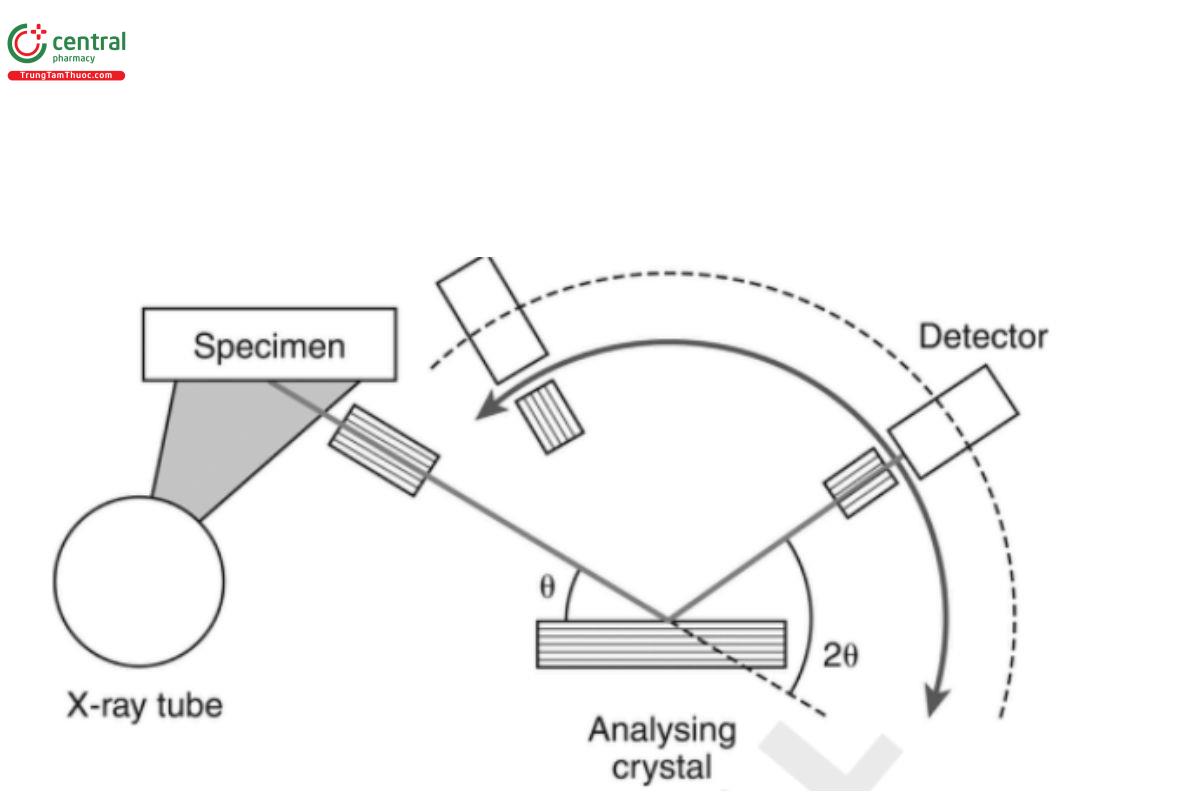
Figure 2. Schematic diagram of a wavelength-dispersive XRF spectrometer, indicating the main components. 

5.1 X-Ray Tube 

The two most important components of an X-ray tube are the lament (used as a cathode) and the anode. The lament is the source of electrons, which are accelerated to the anode material by a strong electric eld between lament and anode. Upon impact with the anode, the electrons can gradually lose their kinetic energy, generating heat and a continuous spectrum of X-ray radiation in the process. Alternatively, when the electrons ionize atoms from the anode, the resulting vacancy can decay by emitting characteristic X-ray radiation. The total spectrum of an X-ray tube thus consists of the characteristic lines of the anode element (which is discrete in nature) superimposed on a continuum. Note that the continuum radiation, scattered by the specimen, is the main source of the background observed in XRF analysis. 

5.2 Primary Beam Filter 

Most X-ray spectrometers are equipped with one or more programmable beam filters. These filters are thin metal foils (typically between 50 and 1,000 microns in thickness) that are mounted on a mechanical device that can move a particular filter in the path of the primary beam. The main purpose of the primary beam is to eliminate the characteristic lines of the X-ray tube anode. If for example a rhodium anode tube is used, a significant part of the incident rhodium X-rays will be scattered by the sample. The fraction that is coherently scattered cannot be distinguished from rhodium lines that are created by atoms in the sample. In such a case, to allow for analysis of rhodium in the sample, the primary beam filter is used to prevent characteristic lines from the X-ray tube from reaching the sample. Another application of beam filters is the reduction of background in certain energy ranges. The lower limit of detection can be improved in cases where the background intensity is significant. However, the use of primary beam filters also leads to a degradation of sensitivity, and care must be taken to achieve optimum setup conditions. 

5.3 Wavelength-Dispersive X-Ray Fluorescence Spectrometry 

5.3.1 principle of operation—bragg's law 

As the name implies, the wavelength-dispersive spectrometers employ an X-ray monochromatizing strategy, using Bragg's Law of Diffraction, to split the X-ray spectrum into its individual components (or rather, narrow energy bands): 

nλ = 2dsinθ [13] 

where n is the order of reflection; λ is the wavelength of the photons considered; d is the spacing of the crystallographic planes, and θ is the angle of incidence (and reflection) with respect to the crystal's plane. In the vast majority of applications, the first  order (n = 1) is used. For diffraction of photons with wavelength λ to occur, the angle θ must be selected such that the product of 2dsinθ equals λ. Bragg's Law can be viewed as the requirement for positive interference of X-ray photons. Consider a monochromatic and parallel beam of X-rays of a specific wavelength λ with electrical vectors of equal amplitude in phase along any point of the direction of propagation. This beam is incident on a crystal at an angle θ. The beam is scattered in all directions. However, constructive interference only occurs in those directions for which the phase relationship is conserved. This happens at an angle θ for incident rays 1 and 2 (see Figure 3), for which the path difference AB + BC is equal to an integer number of wavelengths λ. The integer n refers to the order of the diffraction. The most intense diffraction peaks— and thus the highest measured intensity—can be obtained when n = 1 (first order). Higher-order diffractions with n = 2, 3, or 4 do occur, but the efficiency is low. 

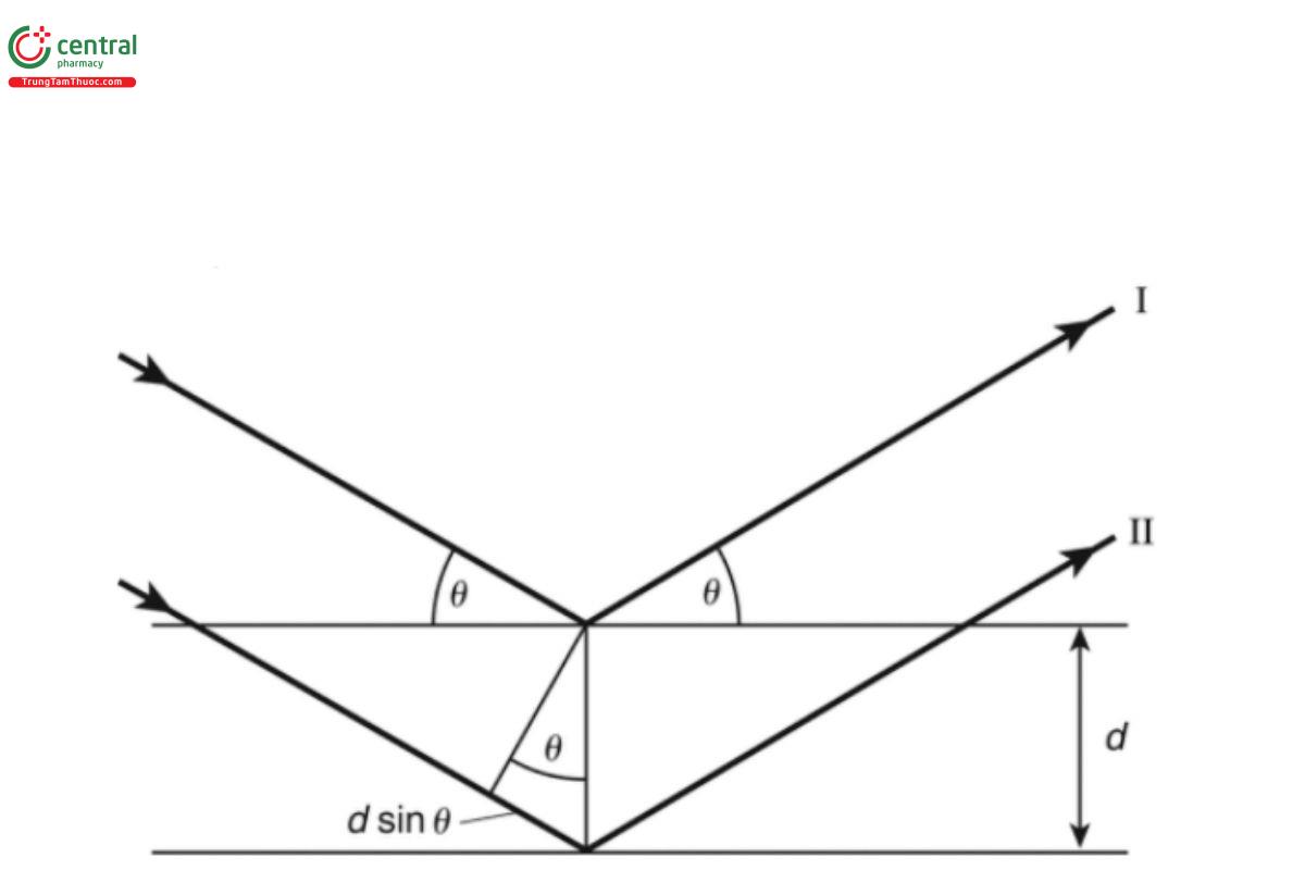
Figure 3. Geometry involving Bragg's law. 

5.3.2 Dispersion 

The dispersion of a WDXRF instrument can be calculated by differentiating Equation [13] as follows: 

dθ /dλ  = n/ (2d cos θ)  [14] 

Dispersion is a measure of the angular separation between peaks corresponding to two different wavelengths. A larger value for the dispersion indicates a larger angular separation, thus a smaller (potential) overlap between photons of slightly different wavelengths. Decreasing the 2d spacing is an obvious way to improve on angular dispersion; the 2d spacing is, however, determined by the crystal used. For most of the wavelength range, there are at least two crystals available; the one with the smaller spacing offers the better angular separation, but typically this involves a loss of intensity. Well-defined crystals with known 2d spacing are used as monochromators. A list of commonly used crystals appears in Table 3. 

Table 3. Commonly Used Monochromators in WDXRF 

Dispersion only describes the angular separation between two peaks; it does not describe the width of the peak, which is typically referred to as resolution (in other forms of spectrometry) and is calculated from the full width of the peak at half height. The actual resolution from the detector system has no discernible influence on peak separation. 

The choice of crystal and angle of the detector relative to the crystal determine which elemental X-ray lines may enter the detector. The main task of the detectors in WDXRF is reduced to counting photons with a known energy, as the use of the monochromator crystal thus separates the selection of the wavelength of the photons from the actual counting. 

5.3.3 Detectors for wdxrf 

Gas-filled detectors: Gas-filled detectors consist of a cylindrical volume filled with a noble gas such as argon (Ar) or krypton (Kr), and a wire running through the center of the detector (see Figure 4). 

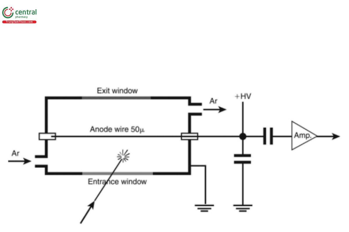
Figure 4. Schematic diagram of a flow counter. 

An incoming photon (represented by its energy hν) can remove an outer (valence) electron of one of the inert gas atoms. For an argon- filled detector: 

Ar → A⁺ + e⁻  [15] 

The energy required for the ionization, e_i, depends on the element; for argon (Ar), about 26 eV is required to create an ion-electron pair.  The total number of such primary ionizations, n_p, caused per incident photon with energy, E, can then be calculated using  

np =E/e_i [16] 

The electric eld between the wire and the outer body will cause the electrons to accelerate toward the anode wire. The positive ions, on the other hand, will migrate toward the housing. The resulting electric eld gives rise to a cascade of ionization events. The result of this cascade effect is as follows: for each of the individual electrons originally created by the incident photon, many more electrons are nally collected at the anode wire (this is called the gas amplification factor and is typically around 10⁴ to 10⁶), creating a voltage drop that is then processed by the counting electronics. 

The entrance window should absorb as few of the incoming photons as possible, because any photons absorbed into the window are lost from the counting circuit, thus reducing the sensitivity. Large windows with low attenuation for long wavelengths can be made from stretched polymers, such as polyethylene or polyester, coated with a conductive material at the interior of the counter to provide for a homogeneous electric eld. Such thin windows need a mechanical support to withstand the pressure difference caused by the vacuum in the spectrometer chamber. The collimator is usually preferred as a support because it will also reduce the amount of radiation that is scattered from the crystal or the multilayer. 

On the other hand, the polymer windows have small pinholes. These pinholes allow the counting gas to gradually leak away. Such detectors would have only a very short lifetime before the counting gas leaked away or became so contaminated that it would effectively render the detector useless. To compensate for the leaks, a constant flow of counting gas is used, the excess of which is vented away out of the spectrometer chamber; such detectors are therefore called flow proportional counters (or gas flow detectors). Only a fraction of this flow is leaking into the spectrometer chamber, whereas the remainder is leaving the detector through a tube and is vented into the atmosphere. It is essential for the overall stability of the spectrometer that the pressure and temperature of the gas are kept constant. Hence, most instruments are equipped with a gas-density stabilizer. 

Gas flow proportional counters are the preferred counters for the detection of X-rays with very long wavelengths in wavelength-dispersive spectrometers. The counting efficiency of the gas-filled detectors is determined by the absorption in the entrance window and the capture efficiency (absorption of the incident radiation) of the counting gas for the wavelengths of interest. The capture efficiency depends on the path length available within the detector, the composition of the counting gas, and its pressure. The absorption properties of the window determine the efficiency of the detector at the long wavelengths, whereas the absorption properties of the gas determine the efficiency at the shorter wavelengths. Considering the typical dimensions, the nature of the gas, and the pressure, the absorption of the gas as function of the wavelength of the incident photon can be calculated. Around wavelengths of 0.2–0.3 nm, about half of the incident photons are not absorbed, reflecting a low efficiency. This is the main reason why sequential WDXRF instrumentation is equipped with more than one detector. 

Scintillation counter: WDXRF instruments are generally fitted with a scintillation counter for the detection of shorter wavelengths for which the gas proportional counter is less efficient. The operation of the scintillation counter is based on two distinct stages: a scintillation crystal and a photo-multiplier tube (see Figure 5). 

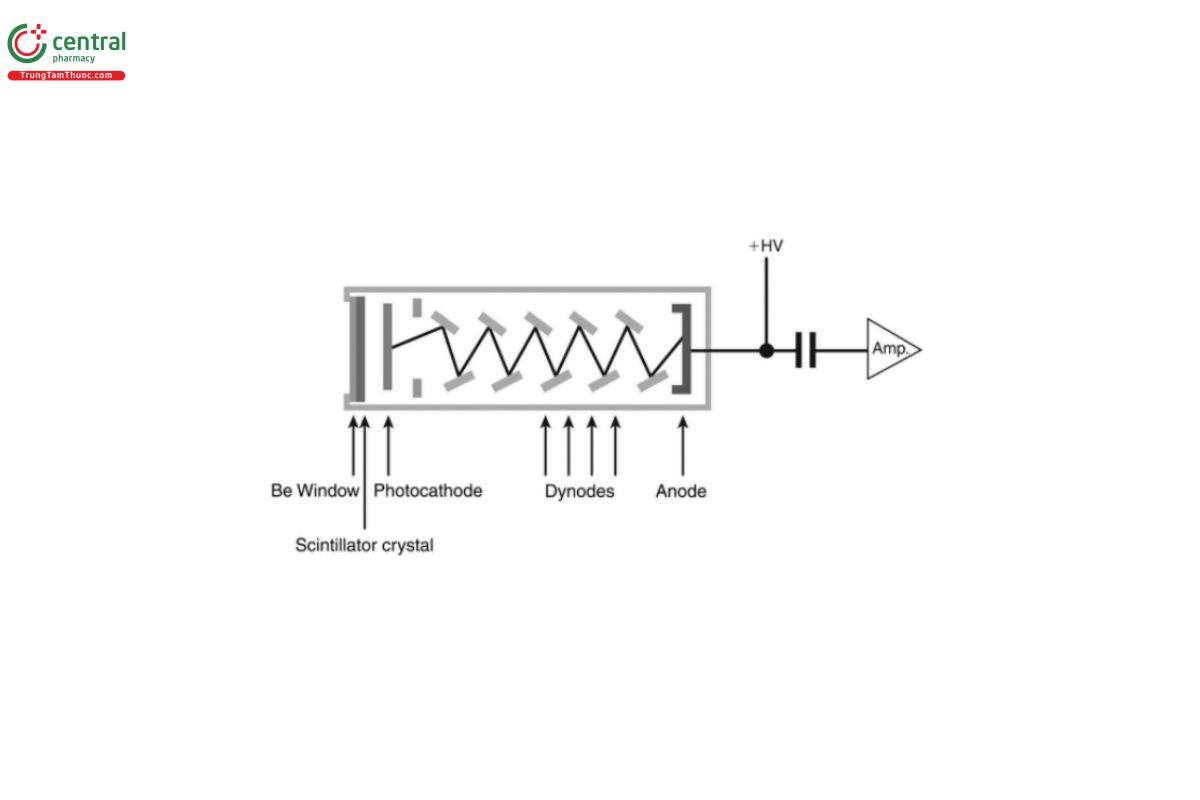
Figure 5. Schematic diagram of a scintillation counter. 

In the first  stage, the incoming photon is absorbed by a “scintillator crystal”. A scintillator is a material that emits light when it is excited by ionizing radiation, such as X-rays. Many different scintillator materials exist, with different properties regarding radiation hardness, operating temperature range, decay times, optical properties, and other properties. The most commonly used scintillator material in WDXRF instruments is a sodium iodide (NaI) crystal, doped with thallium (Tl). The scintillating crystal is optically coupled to a “photo-multiplier”, which consists of a photo-cathode and a series of dynodes. In the second stage, upon impact by a photon, the photo-cathode releases free electrons. These are then accelerated toward a series of dynodes. At each dynode, the impact of the electrons generates more electrons. If 10 dynodes are used, the total amplification provided is about a factor of 106. 

The counting efficiency of the scintillation counter is largely determined by the thickness of the sodium iodide thallium [NaI(Tl)] crystal. The counting efficiency for a 3-mm-thick crystal is better than 99% for wavelengths of 0.05 nm and longer. This allows the detection of high energy photons such as Sn Kα with high efficiency. 

The production of light photons is higher in the scintillation detector than the number of electron-ion pairs created in a flow counter; this should lead to a better resolution. However, this advantage is cancelled out by the low yield of photo-electrons by the photo-cathode, where less than 1 electron is freed for every 10 incident light photons. Compared to the gas-filled counters, the resolution of a scintillation counter is worse. 

The use of the WDXRF technique (typically with power in the kW range) for organic matrix sample analysis is limited because heat generated by the X-rays may be  sufficient to induce significant specimen alteration, such as browning or burning of the sample surface. Furthermore, even if the sample is measured for a very short time by WDXRF, the heat imparted to the sample surface may induce the loss of volatile elements [e.g., mercury (Hg) and Selenium (Se)]. The WDXRF technique is, however, perfectly suited to measure inorganic materials that can withstand elevated temperatures. Examples of common inorganic materials that are suitable for WDXRF measurement are calcium carbonate (CaCO₃) and sodium chloride (NaCl). 

5.4 Energy-Dispersive X-Ray Fluorescence Spectrometry 

5.4.1 Principle of operation 

The energy-dispersive XRF technique typically involves simultaneous detection of photons of different energies that are emitted by the atoms in the sample. The detector determines both the photon's energy and the intensity, which is the number of photons per unit of time. To provide adequate resolution for distinguishing between characteristic lines and overlapping lines from other elements, most EDXRF instruments are equipped with a high-resolution detector and a multi-channel analyzer (MCA). The MCA essentially provides a histogram representation of the spectrum. High-end instruments use sophisticated calculation (deconvolution) algorithms to identify the peaks (i.e., to establish the presence of certain elements) and to obtain intensity data from the histogram. EDXRF is theoretically a simultaneous technique because it measures the complete spectrum in a single counting phase. However, significant improvements in performance can be achieved by measuring the sample using two or more different excitation conditions, each optimized for a certain energy range. 

Compared to WDXRF, the design of an EDXRF spectrometer is much simpler because it lacks a high-precision goniometer and the associated collimators. The positioning of the detector relative to the sample is very simple; the most obvious requirement is that there should not be a direct path between the anode of the X-ray tube through the entrance window of the detector onto the active body. Distances between the X-ray tube window and specimen, and between the specimen and detector entrance window, can be small, in the order of 1–2 cm. Furthermore, as only limited collimation is required, the angle of acceptance of the photons from the specimen can be quite large. Low-power X-ray tubes with ratings up to 50 W are used. Because of the inherent simplicity of their design, wide variation of systems with varying capabilities exists. A typical spectrum on an energy-dispersive spectrometer is shown in Figure 6. The energy on the horizontal axis increases from left to right. The peak shape is nearly perfect Gaussian. 

Figure 6. Energy-dispersive spectrum of a brass specimen. From left, the peaks are due to Cu Kα, Zn Kα, Cu Kβ, and Zn Kβ. The horizontal axis is energy and the vertical axis is in counts per channel. This spectrum was recorded at 75,000 cps with 50 kV and an Ag primary filter to reduce the background. The full width at half maximum (FWHM) is about 165 eV at the Cu Kα peak. 

5.4.2 Detectors 

The resolution of the detector system determines both the peak width (expressed as FWHM) and the peak separation. Systems may be equipped with gas-filled, solid-state, or semi-conductor detectors. The three most common solid-state detectors used are the following:

• Liquid nitrogen-cooled silicon-lithium drifted Si(Li) 
• Liquid nitrogen-cooled germanium detectors, such as the LeGe and HPGe 
• Detectors based on intrinsic silicon, such as the PIN (positive, intrinsic, and negative) detector and the SDD (silicon drift detector). 

The first  two types of detectors allow for high photon-capture efficiency but require relatively bulky, well-insulated containers (Dewar) for the liquid nitrogen. These detectors are generally rather large, which improves sensitivity, and thick, which improves capture efficiency for high-energy photons. They are typically found on floor-standing equipment. Bench-top systems are equipped with detectors that are based on intrinsic silicon. These types of detectors do not require cooling to temperatures as low as the other two categories; temperatures between −25° and −15° are acceptable. Peltier-cooling or electro-thermal cooling is  sufficient to reach those temperatures. The detectors are smaller and thinner than their bulk siblings. Older equipment might still be using so-called PIN detectors, but all of the newer equipment tends to be equipped with an SDD. The SDDs have much better resolution and can be used at much higher intensities than the PIN detectors, which are typically limited to about 220 eV at Mn Kα. The SDDs combined with state-of-the-art electronics have a resolution (expressed as FWHM) of better than 145 eV at Mn Kα. This is comparable to liquid nitrogen-cooled semi-conductor detectors. A word of caution is required as the resolution worsens with increasing count rate or intensity. Most manufacturers therefore specify resolution at an impractical, low count rate of 1,000 or 2,000 cps. 

5.5 Polarized X-Ray Spectrometry 

5.5.1 Principle of operation 

The most elaborate EDXRF spectrometers use polarization or a secondary target to modify the spectral distribution of the X-ray source; the aim is to reduce, or ideally eliminate, the intensity of the continuum background. This effort is a logical consequence of Equation [3]. Due to the fact that the major component of the background is scattered tube radiation, one method of preventing radiation from the X-ray tube from reaching the detector system is the use of polarized radiation. These systems have applications in the analysis of, for example, residues of palladium (Pd) catalyst in some pharmaceutical ingredients. 

5.5.2 Polarized radiation and polarizing target 

The orientation of the electric eld vector, E, of the photons generated in an X-ray tube is random but always perpendicular to the direction of propagation. Using a Cartesian coordinate system, with the z-direction coinciding with the direction of propagation, the two components of the electric eld vector in the x-direction (denoted by E ) and y-direction (E ) are identical and obey the following relationship: 

 E_x² =   E_y² = 1/2 . E² [17] 

The component along the axis of propagation, E_z is zero; this is because electromagnetic radiation is a transverse wave. After coherent scattering in the yz plane, the eld vector of photons traveling in the y direction, E_y, is also reduced to zero. This beam of photons, all with their electric eld vector parallel to the x-direction, is directed at the sample and interacts in the usual way. The photons cause ionizations and can be scattered, but they cannot be scattered in the direction along the x-axis, because the electric eld vector cannot have a component parallel to the direction of propagation. If the detector is now placed somewhere along the x-direction (still in the same frame of reference), the background is significantly reduced because the main contribution (i.e., scatter from the incident radiation) is absent. The process is inefficient because there is no active polarization; it is entirely achieved by suppressing one component of the electromagnetic wave, thereby significantly reducing its intensity. Therefore, high-power X-ray tubes are used. 

5.5.3 Secondary targets 

The use of secondary targets in energy-dispersive spectrometry has been widespread for high-power instrumentation. The aim is to reduce the background, thus improving the lower limit of detection. When electrons decelerate, they generate Bremsstrahlung of a continuous nature; however, photons do not generate Bremsstrahlung. The principle behind an instrument equipped with secondary targets is to use a classic X-ray tube to provide a beam of X-rays (including the troublesome continuum) and direct it at a secondary target, which is typically a metal. The radiation emanating from the secondary target will consist of the very intense characteristic radiation corresponding to the nature of the target and scattered continuum. The intensity of the scattered background is relatively low, especially when the target material is a metal of medium-to-high atomic number. There is no additional continuum created by the incident photons, but a tiny contribution to background radiation is created by the high-energy photo-electrons. The radiation from the secondary target is directed at the sample for excitation purposes. The spectrum from the sample is composed of the characteristic lines from the elements present, the scattered characteristic radiation from the secondary target, and the concomitantly scattered continuum from the tube. The latter contribution is very weak because it has been subjected to two scattering events, one at the secondary target and another one at the sample. If the instrument is equipped with a selection of secondary targets, then significant improvements in the lower limit of detection can be obtained. The two-step process requires a higher-power X-ray tube to get the same ux at the sample when compared to direct excitation, so it is generally not incorporated into bench-top instrumentation. Currently, secondary targets are often used in combination with polarization targets. This combination is straightforward, because both types of targets can use the same geometrical arrangement. 

5.6 Total reflection X-Ray Fluorescence Spectrometry 

Another variety, total reflection X-ray fluorescence (TXRF, also sometimes abbreviated to TRXRF), specializes in the analysis of infinitely thin and extremely homogenous samples derived from liquids. Typically, TXRF instrumentation employs an X-ray source, which is directed at the sample under a very small angle with respect to the surface. The detector is typically placed above the sample at a 90° angle. The TXRF technique commonly uses internal standards (mixed into the unknowns) and geometrical relationships to determine elemental concentrations. 

6 QUALITATIVE XRF ANALYSIS 

This section applies to both WDXRF and EDXRF. 

6.1 X-Ray Spectra 

Qualitative analysis by means of X-ray fluorescence is relatively simple because the characteristic line spectra of the elements are simple and are not affected by chemical bonding; i.e., these spectra are truly elemental. For qualitative (and quantitative) analysis, the main lines are those from the K- and L-series. The K-lines result from electron transitions after one of the K-electrons has been expelled. Due to quantum mechanical selection rules, not all transitions are allowed. Transitions from the L-shell to the K-shell are limited to transitions involving L2 and L3, as radiative transitions between the L1-shell and K-shell are forbidden. These transitions are the most probable, leading to the most dominant line in the spectra. For most elements, the energy difference between the L2-shell and L3-shell is rather small (in the order of a few eV), so the emitted lines are typically not separated and simply considered a doublet. Radiative transitions from M- and N-shells to the K-shell are also occurring. These give rise to a more complex part of the K-spectrum. In practice, however, only the Kβ_1,3 doublet (resulting from transitions between M3 and K and M2 and K) is of importance. The relative intensity between the Kα and the Kβ varies from 1 in 1,000 for sodium (Na) to 1 in 6 for plutonium (Pu), with the Kα always being the most intense line of the series. 

The Kα-line is generated by an electron transition from an electron in the L3 shell, following the removal of a K-shell electron. The Kα-line is the most dominant line in an element's series. The K electrons of an element, however, have the highest binding energy of all electrons in the atom, and thus are only excited by high-energy incident photons. This is generally not a problem for the low- and middle-atomic number elements, but excitation of the K-lines of elements with atomic numbers above 50, for example, might not be possible, as the excitation potential is higher than the maximum operational voltage on most X-ray tubes. 

Whereas the K-line spectra are typically limited to two lines only, the situation for the L-series spectra is more complicated. For lead (Pb), a total of 46 L-lines are listed in Bearden [2]. Many of these are weak, or are doublets. For qualitative analysis, not all of these lines are to be considered. In all cases, it is important to realize that if the Kβ is visible, then the Kα must be visible too and must have a higher intensity. 

6.2 Qualitative Analysis 

Qualitative analysis typically consists of a few simple steps. After the spectra have been collected, the background is subtracted. This background subtraction can be done in a separate step, or it can be done in conjunction with a peak search algorithm. A fraction of these photons propagate in the direction of the analyzing crystal (WDXRF) or directly to the detector (EDXRF). Next, a peak search is performed, and nally, these peaks are identified, i.e., each is attributed to a particular element. efficient algorithms for qualitative analysis look for the presence of each element, rather than trying to identify each peak. This is different from X-ray diffraction, where each peak is checked for a match with a phase. In this method, the peak search is performed first. Then, for each element, the presence of the Kα_1,2 -doublet is verified. If this line is found in the spectrum, then the weaker lines of the same series (Kβ_1,3 and Kβ₂ ) are investigated. Note that all characteristic lines in the same series should appear, except in cases where the intensity of a weaker line is similar to the intensity of the background. For elements with higher atomic numbers where the K-lines are not excited (or not detected due to limitations in detection hardware) the process starts with the L-line spectra. The intensity ratios of, for example, Kα to Kβ are listed in several databases [8,9]. The tabulated ratios are for the “isolated” atom; they reflect the intensities as obtained from an atom without any matrix effects. These ratios can be corrected quite easily for matrix effects, even in the case of overlapping lines. Only elements that are present at trace levels (with intensities comparable to the standard deviation of the background intensity) are usually deemed “not present”. Note that, in principle, line interference between elements is not much of a problem in qualitative analysis; this is due to the fact that in qualitative analysis, many more data points that cover alternative lines are available. Hence, establishing the presence of elements is not impacted as much as one would suspect. Also, in energy dispersive spectrometry, where the line overlap is most severe, adequate corrections can be performed because the peak shape is rather well known. 

7 QUANTITATIVE XRF ANALYSIS 

7.1 Selection of Analytical Line 

The characteristic emission spectra of most elements contain several lines. The choice of an analytical line for a given element is largely dependent on three factors: the concentration of the element in the sample, the potentially interfering lines, and the excitation capabilities of the spectrometer. In most cases, the Kα emission line of an element is preferred. When the excitation of the K-lines is not possible due to limitations of the tube and/or generator, the use of L-lines, with their lower energy, is necessary. Use of the Lα-line (when the Kα-line is not excited) does not involve much of a detriment because for those elements, the intensity of the L-lines is quite high. Also, the detection efficiency of the L-line photons is then much higher than that of the high-energy K-lines of the same element. For elements with high atomic numbers (i.e., Z larger than about 72), the Lβ offers a very good alternative to the Lα and these lines have comparable sensitivities. 

In general, on a typical WDXRF instrument, all elements with atomic numbers up to 56 are measured on their Kα-line. For elements with higher atomic numbers, the Lα-line is used. For EDXRF spectrometers equipped with SDD-using generators (and tubes) with a maximum voltage of at least 30 kV, K-lines are available to measure for elements up through about Z = 47; the L-line spectra are used for all elements with higher atomic numbers. The exact point at which the switch over occurs between the K-line and the L-line spectra depends on factors such as the application and the anode material of the X-ray tube used. 

Quantification procedures are carried out using routine spectroscopic techniques involving the measurement of blanks and standards of varying elemental concentrations. The measured intensities are then corrected for background and for line overlap, if required. In a number of cases, a straightforward linear relationship between the intensity of the analyte and its concentration can be established. This is especially the case with low concentrations in a constant matrix. In the more general case, however, corrections for matrix effects are required. Matrix effects are not the limiting factor in the precision of the nal analysis, but they must be accounted for in order to obtain an accurate measurement. 

7.2 Matrix Correction Techniques 

7.2.1 Origin of matrix effects 

XRF is typically applied to condensed samples, without resorting to dissolution of the sample in an abundance of acids or other solvents. Thus, the samples remain concentrated, in contrast to many other techniques. Because of this, the XRF technique is prone to matrix effects, in that the relationship between the intensity of a particular analyte and its concentration is generally not as simple and straightforward as with diluted specimens. With the latter, this relationship between concentration and intensity is often expressed as a straight line. However, the presence of other elements at high concentrations can cause deviations of this straight-line relationship. The physics of X-ray emission and detection is well understood and relatively simple for bulk materials, and this provides a solid theoretical basis for a mathematical description of matrix effects. Matrix effects can thus be described accurately and correctly using a variety of mathematical techniques, and several methods have been developed to address them. Two main matrix effects can be distinguished and are discussed below— absorption and enhancement. 

Absorption: Absorption as a matrix effect occurs when the matrix elements and the analyte element have different absorption properties for the characteristic radiation of the analyte. If the mass attenuation coefficient of one or more of the matrix elements is larger than the mass attenuation coefficient of the analyte, the matrix will absorb more of the analyte radiation than expected and the measured intensity of the analyte will be lower. This results in a concave calibration curve. If, on the other hand, the absorption of the matrix elements is lower, a higher intensity of the analyte will be measured and a convex calibration curve will be observed. Absorption as a matrix effect can be large, reducing the intensity by as much as 100% (and more) or “increasing” it by as much as 10%, depending upon the analyte and matrix elements. The magnitude of the absorption effect depends on the wavelength of the analytical line considered and the composition of the specimen. In a given specimen, the absorption effect can be significant for the characteristic line of one analyte and rather insignificant for another. The absorption effect can also differ significantly for the same analyte when measured on two different characteristic lines. 

The three processes that cause absorption are the photo-electric effect, the coherent scatter, and the incoherent scatter. In general terms, photons with a given energy will be absorbed more with increasing atomic number of the absorbing element. Also, the absorption by a given element decreases in a steady, smooth manner when the photon energy increases. However, when the photon energy exceeds the binding energy of electrons in an inner shell, the photo-electric effect (see 3.1 Ionization and the Photo-Electric Effect) causes an increase in absorption. This leads to discontinuities in the absorption curve at energies corresponding to the binding energy of the electron levels. These discontinuities are called absorption edges; the energy at which the absorption edge occurs is equal to the binding energy of the electron shell concerned. 

Enhancement: Enhancement as a matrix effect is the process whereby the characteristic radiation of matrix elements is absorbed by atoms of the analyte, subsequently causing characteristic radiation of the analyte. The intensity of the analyte is thus enhanced, which leads to concave calibration curves. For a given analyte, all characteristic lines from the same series are enhanced to the same degree. This is because the root cause of the enhancement is the photo-electric absorption of radiation from matrix elements. The effect of enhancement is typically smaller than that of absorption. It is most pronounced in alloys of the first-row transition elements, where it can reach 25%. In many other applications, the enhancement effect is smaller, but is still important enough to warrant consideration and correction. 

7.2.2 Fundamental parameter methods 

The physical processes involved in absorption and excitation in XRF are well understood and easy to model mathematically. All entities required are listed in a variety of tables and databases. The calculations were previously tedious and time consuming, but with the current computing power available, the calculation effort is no longer an obstacle. Fundamental parameter methods are based on the underlying physical processes governing X-ray fluorescence, including the specifics of the instrument's geometry, the anode material of the X-ray tube, the voltage on the tube, and the composition of the specimen. The derivation of the equations is beyond the scope of this chapter, but is addressed by Criss and Birks [10] and Shiraiwa and Fujino [11]. 

7.2.3 Compton correction 

The use of Compton scattered radiation as a means to correct for matrix effects (as well as for variations in sample preparation) has been described by Reynolds [12] and Taylor and Andermann [13]. The Compton correction is based on the fact that the intensity of incoherent (or Compton) scatter is inversely related to the mass attenuation coefficient of the sample. In practice, a high-energy characteristic line from the tube anode is used. Measuring the intensity of the Compton scattered tube line thus reveals information about the absorption properties at the wavelength of the Compton scattered line. At first  glance this seems to be of limited use, but in the field of X-rays, values of the mass attenuation coefficients for the same sample at different energies/wavelengths are proportional. This relationship, and the fact that absorption is the major source of matrix effects, explains why the Compton correction is a powerful correction method in a variety of matrices. 

It is, however, not generally applicable and will fail in cases where there are significant absorption edges between the wavelengths of the Compton scattered radiation, at the wavelength of the analytical line used. The correction is based on the relationship between Compton scatter and the sample's absorption properties, and it does not correct for enhancement. 

7.2.4 Influence coefficient algorithms 

Matrix correction methods based on influence coefficients have the general format: 

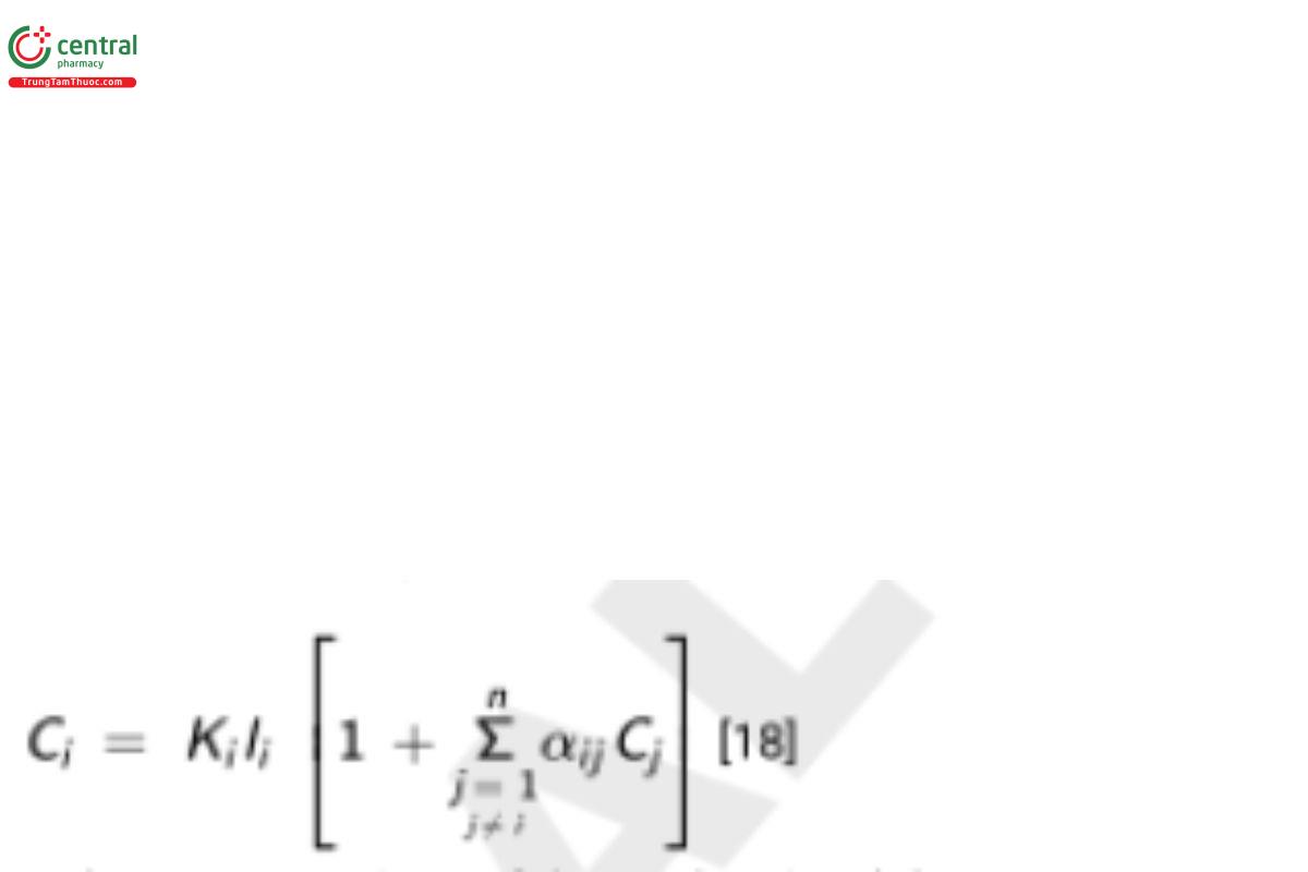
(based on Lachance and Traill [14]) where C and C are the concentrations of the analyte i and the interfering element j, respectively, and α i j ij is the influence coefficient, expressing the influence of interfering element j on the analyte i. All concentrations are expressed as weight fraction. The summation in Equation [18] has n − 1 terms, for a sample consisting of n elements or compounds; this is a simple yet essential feature of the algorithm. The same set of equations with n terms in the summation would lead to a homogeneous set of simultaneous equations, from which only ratios rather than absolute values could be derived. 

Because the sum of the concentrations of all elements (whether they are measured or not) in a specimen always totals 1, one element can be eliminated. Most influence coefficient algorithms in software are based on this equation, however they may differ in how the values of the coefficients are calculated. 

7.2.5 Empirical influence coefficients 

Lachance and Traill [14] indicate that the value of the coefficients should be calculated from theory, but they only provide a simple and limited method that fails to consider enhancement or the polychromatic nature of the incident beam. Therefore, in many cases the coefficients were determined using multiple regression methods. Many early variations on influence coefficient algorithms were based on regression techniques that were used to calculate the value of the coefficients. However, the use of regression methods should be discouraged as they often lead to overly optimistic indications of precision and then often fail during validation. This is especially problematic if not enough certified reference materials are used in the calibration. The minimum number of standards used should be at least 3 times the number of parameters. Each of the influence coefficients whose value is determined by regression consumes one degree of freedom, as does the determination of slope and intercept. 

The total number of parameters to be determined can grow rapidly for a single analyte. For example, assume that there are three interfering elements, and thus with slope and intercept, a total of ve parameters need to be determined. This requires a minimum of 15 independent and uncorrelated standard samples. Note that replicates of the same standard sample do not count as individual samples, but instead count as a single one; this is a common source of error. Also, care must be taken to ensure that the standards are uncorrelated. This implies that a series of dilutions from a given standard cannot be used when empirical influence coefficients are to be determined. In a dilution series, two (or more) components A and B increase (or decrease) in the same direction. Thus the effect of component A on the intensity of the analyte cannot be distinguished from component B's effects, leading to erroneous values for the influence coefficients. 

7.2.6 theoretically calculated influence coefficients 

De Jongh [15] was the first  to publish a method detailing the calculation of influence coefficients, using theory only to eliminate a compound other than the analyte. The algorithm is still in common use today. The eliminated compound can be the non-fluorescing matrix, such as cellulose, or the matrix when its concentration is not certified. Note that the concentration range over which the algorithm delivers precise results is rather limited when the matrix effects are severe. This is a direct consequence of the fact that the values of the influence coefficient are calculated for a particular composition of the sample. For routine analysis involving relatively limited concentration ranges, the algorithm delivers excellent results. In contrast to the situation where the values of influence coefficients are determined by regression (see 7.2.5 Empirical influence coefficients) it is feasible to calibrate using dilution series. 

7.3 Measurement Method Development and Calibration 

7.3.1 Overview 

Once the elements of interest have been identified, the spectrometer measurement parameters must be set appropriately. This involves determining the “ideal” measurement conditions for each element. The list of parameters to be selected for each analyte can include, for example, the voltage and current on the X-ray tube, the crystal and the collimator (WDXRF), the type of primary beam filter (if used), and other parameters. For elements that are similar in atomic number, the settings will be quite similar. The precision of XRF measurements is theoretically limited by the CSE. It has been shown that the CSE of a measurement of N counts (photons) is given by the square root of N. It is a generally accepted practice to determine the measurement times that obtain an acceptable CSE for each element of interest. Sample preparation errors and the CSE are the largest contributors to the total analytical precision. Once the measurement time has been established, it is important to ensure that the background positions and methods for peak fitting are also appropriate. 

After the net intensities of the elements of interest have been obtained from a suitable number of reference standards, a calibration can be performed. For low concentrations of analytes in an otherwise constant matrix, linear regression may be appropriate. When evaluating specimens with higher concentrations of analytes, the calibration also involves correction for matrix effects. The fact that the EDXRF technique is not capable of measuring the organic constituents of an actual pharmaceutical composition is of little concern. This is certainly true if the composition of the matrix is constant, and if the total content of measurable elements is low. But if these two conditions are not satisfied, the difference in scattering properties can result in calculation errors if not corrected. Fortunately, there are numerous strategies that accommodate these differences, such as the fundamental parameters method or the Compton correction method. The nature of matrix effects, as well as methods to correct for them, have been discussed above. The application of these methods to calibration and analysis of unknowns will be discussed in the sections below. 

7.3.2 Calibration using influence coefficient algorithms 

Calibration using influence coefficients is rather straightforward. Once the values for the coefficients have been calculated for each of the standard samples, the summation 

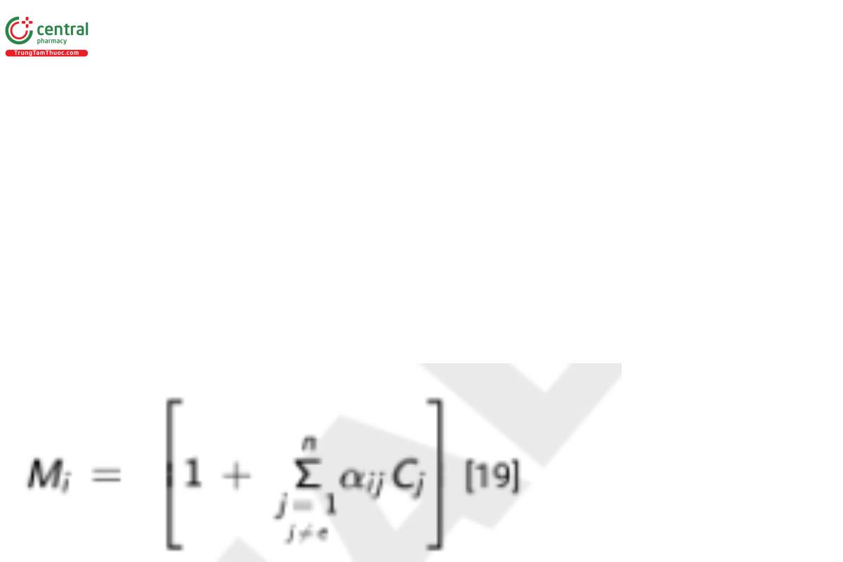
can be calculated where for standard samples, the concentrations, C_j, are known. The value of M_i for one standard sample will be different from the value for another standard sample, and it does not matter whether the difference is significant or slight (large or small). If adequate corrections for background have been made, calibration is then represented by 

C_i = K_i I_i M_i [20] 

where the product of the measured intensity, I_i , and the corresponding value for the matrix effect ,M_i, are regressed against the given, known concentration, C_i, to determine the slope, K_i. This equation assumes that the intensity, I_i, is properly corrected for the background. In those cases where the intensity of the background is constant between samples and standards, a slightly modified equation can be used: 

C_i = B_i + K_i I_i M_i [21]  

where B_i is the intensity of the background. In this case, both B_i and K_i are determined by regression analysis. In situations where the background intensity varies significantly between samples, or between samples and standards, proper background correction must be applied to the measured intensities, and the corrected intensities must be used for the calibration. 

7.3.3 Calibration using compton correction 

In this case, both the intensity of the analyte, I_i, and the intensity of the Compton scattered line, I_C, are measured. The intensity of the Compton is inversely proportional to the mass attenuation coefficient [12], or 

M =    1/I_C [22] 

Combining this with Equation [20] leads to 

C_i =   K_i .l_i. (1/I_C) [23] 

The intensity of the analyte and the Compton line are measured on a suite of standard samples and regressed against the analyte concentration to determine the value of the slope of the calibration. A background factor, B , can be determined as well. i 

7.3.4 Calibration using fundamental parameter methods 

The physical processes involved in absorption and excitation during XRF are well understood, and it is possible to calculate the value of the matrix effect based on several factors: the composition of the sample, the type and settings of the tube, the geometry of the spectrometer, and the fundamental parameters: 

M_i = f(C_i , C_j,…,C_n, tube, geometry, fp) [24] 

This value of M_i is calculated for each standard and for each analyte of interest, and then applied in the usual manner. 

7.3.5 Internal standard method 

An alternative to the methods described above is the internal standard method. A fixed quantity of an element s (other than the analyte i) is added to all specimens. The element s is chosen such that it is not present in the specimens, thus ensuring that its concentration is the same for all specimens. In the absence of matrix effects, the measured intensity of its characteristic radiation would also be constant. Any variation in its intensity (other than the variation resulting from the counting statistical error) is attributed to the presence of matrix effects. The idea is to choose the internal standard element s in such a way that the intensity of its characteristic radiation is subject to the same matrix effects as the intensity of the analyte element under consideration. Both intensities—of the analyte and of the added element— increase (or decrease) in proportion to one another depending upon the matrix effect. Equation [22] can be modified for the internal standard element s: 

C_s = K_s I_s M_s [25] 

In this equation, C_s is a constant. Taking the ratio of Equation [20] and Equation [25] and solving for the only unknown, C_i, yields

C =    (K_i.M_i.C_s/ K_s.M_s). (l_i/l_s) [26] 

It is important to note that the terms of the first  fraction in Equation [26] are either all constants (K_i,K_s and C_s) or are proportional to one another (M_i/M_s). Equation [26] can thus be reduced to 

Ci   = K∗iIiIs 

where all of these constants are collated in a single variable K_i *  [27] 

The main challenge in applying this method is the selection of the element to be used as the internal standard. This element must not be present in the specimens (or at most, present at very low levels that will not interfere with the analysis). Also, its characteristic radiation must be subject to the same matrix effects as the analyte(s) of interest, and its emission spectrum should not cause interference. In particular, care must be taken to ensure that the analyte element and the internal standard are both subject to (or both not subject to) enhancement by a matrix element. In the same fashion, when the analyte is in the presence of matrix elements that strongly absorb the characteristic radiation of the analyte, the same should apply to the characteristic intensity of the internal standard element. 

When the samples are organic matrices typical of pharmaceuticals, it is easy to satisfy the essential requirement that the characteristic radiation of both the analyte(s) and the internal standard are subject to the same matrix effects. These organic matrices do not exhibit characteristic radiation of their constituent elements, which makes it easier to find a suitable internal standard element. A simple guideline is to choose an element that is not present in the samples and that has an emission line close to the one of the analyte's (with regard to either wavelength or energy). The characteristic lines themselves do not have to be the same or even from the same series, and the method also works when the analytical line is a Kα and the line of the internal standard is, for example, an Lβ. It must be noted that there is no requirement for the internal standard element to be a pure element. Stable compounds that are easily soluble in a solvent can be used. The solvent is, in many cases, the same as the base material of the specimens and the calibration standards. If more than one internal standard element is to be used, it is recommended that both elements/compounds are added in a single internal standard solution, to minimize errors. 

7.4 System Suitability Criteria 

Performance characteristics that demonstrate the suitability of an XRF method are similar to those required for any analytical procedure. A discussion of the applicable general principles is found in Validation of Compendial Procedures 〈1225〉. 

7.4.1 Limit of detection and limit of quantitation 

The lower limit of detection may be expressed as: 

LLD =  (3.3 ×  CSE) / S    =    (3.3 ×  C/ I_net). √ (I_b/t)  [28] 

with I_net representing the net count rate at the concentration, C; I_b as the count rate of the background; and t_b as the background measurement time. It is noteworthy that the detection limit will improve with the square root of the measuring time. The limit of quantitation can be estimated by calculating the standard deviation of NLT six replicate measurements of a blank and multiplying by 10. Other suitable approaches may be used (see 〈1225〉). 

7.4.2 Long-term stability and drift correction 

Under standard operating conditions, instrumental drift of X-ray spectrometers is less than 1% relative and can be as small as 0.1% relative for high-end instrumentation in well-maintained laboratories over the same time period. To monitor instrument drift, one or more stable sample(s) with reasonable intensities (to minimize the CSE) for the analytes of interest can be measured on a regular basis. It is not necessary to use in-type drift correction samples. It is common to use glassy samples and alloys. Most instruments have drift correction routines within the software, and because XRF is a very robust technique, it may only be necessary to utilize a drift-monitor once per month. However, it is recommended that most laboratories practice drift monitoring more frequently. 

7.4.3 Analysis 

Once a method has been established through the calibration procedure, a sample analysis may be performed. It is essential to ensure that samples and standards are treated in exactly the same manner. This includes specimen preparation and specimen presentation to the instrument. 

7.4.4 Calculations and reporting 

In the event that the free-pressed-pellet sample method is used (i.e., pressed without binder), the spectrometer results represent nal sample concentrations, and no further calculations are required. Similarly, both loose powders (i.e., pure, fine materials) and undiluted liquids measured in disposable sample containers require no further calculation and the spectrometer results represent nal sample concentrations. Any material that has been diluted, such as a liquid or pressed pellet, will require additional calculation. Most modern XRF instrumentation comes with software packages that include calculation functions that accommodate dilution factors and automatically back-calculate sample concentrations. For diluted, pressed-pellet samples, the reported units may be weight % or ppm. The actual units for the concentrations are of little importance, as long as care has been taken to work with the proper conversion factors. If a calibration for liquid samples is setup to deliver results in µg/mL, the nal concentration of a given element can be calculated in µg/g from the solution element concentration in µg/mL. 

8 ADDITIONAL SOURCES OF INFORMATION 

1. Beckhoff B, Kanngießer B, Langhoff N, Wedell R, Wolff H, editors. In: Handbook of practical X-ray fluorescence analysis. Berlin: Springer Verlag; 2006. p. 1–878. 
2. Buhrke VE, Jenkins R, Smith DK, editors. A practical guide for the preparation of specimens for X-ray fluorescence and X-ray diffraction analysis. New York: John Wiley & Sons; 1998. 
3. Greiner W. Quantum mechanics: An introduction. 1st ed. Berlin: Springer Verlag; 1994. 
4. IUPAC. Compendium of chemical terminology (the “Gold Book”). 2nd ed. McNaught AD, Wilkinson A, compilers. Oxford: Blackwell Scientific Publications;1997. [Nic M, Jirat J, Kosata B. XML on-line corrected version available: http://goldbook.iupac.org. Jenkins A, updated compilation; 2006.] 
5. IUPAC. Nomenclature, symbols, units and their usage in spectrochemical analysis–VIII. Nomenclature system for X-ray spectroscopy. (Recommendations 1991). 
6. Jenkins R, Manne R, Robin R, Sénémaund C. Nomenclature, symbols, units and their usage in spectrochemical analysis. VIII. Nomenclature system for X-ray spectroscopy. Pure Appl Chem. 1991;63:735–746. 
7. Jenkins R, Manne R, Robin R, Sénémaund C. Nomenclature, symbols, units and their usage in spectrochemical analysis. VIII. Nomenclature system for X-ray spectroscopy. X-Ray Spectrom. 1991;20:149–155. 
8. Klockenkämper R. Total-reflection X-ray fluorescence analysis. New York: John Wiley & Sons; 1996. 
9. van Grieken R, Markowicz A, editors. In: Handbook of X-ray spectrometry. Second edition: revised and updated. New York: Marcel Dekker; 1968. 
10. Vrebos B. X-ray fluorescence analysis. In: Cullen M, editor. Atomic spectroscopy in elemental analysis. Boca Raton, FL: Blackwell Publishing Ltd.; 2003. 
11. Willis JP, Duncan AR. Understanding XRF spectrometry. 2nd ed. Vol 1. Almelo: PANalytical B.V.; 2013. 

9 REFERENCES 

1. Veigele WJ. In: Robinson JW, editor. Handbook of spectroscopy. Cleveland OH: CRC Press, 1974. p. 28. 
2. Bearden JA. X-ray wavelengths. Rev Mod Phys. 1967;39:78–124. 
3. Willis JP, Duncan AR. Understanding XRF spectrometry. Vol 1. Almelo: PANalytical B.V.; 2008. 
4. Greiner W. Quantum mechanics: an introduction. 4th ed. Berlin: Springer Verlag; 2001. 
5. Bambynek W, Crasemann B, Fink RW, Freund HU, Mark H, Swift CD, Price RE, Venugopala Rao P. Rev Mod Phys. 1972;44:716–813.
6. Hubbell JH, Trehan PN, Singh N, Chand B, Mehta D, Garg ML, Garg RR, Singh S, Puri S. A review, bibliography, and tabulation of K, L, and higher atomic shell X-ray fluorescence yields. J Phys Chem Ref Data. 1994;23(2):339–364. 
7. Wolska J, Vrebos B, Brouwer P. Analysis of fuels, lubricants, and greases using X-ray fluorescence spectrometry. J ASTM Int. 2006;3(1):98–107. 
8. Venugopala Rao P, Chen MH, Craseman B. Atomic vacancy distributions produced by inner-shell ionization. Phys Rev A. 1972;5:997.
9. Elam WT, Ravel BD, Sieber JR. A new atomic database for X-ray spectroscopic calculations. Rad Phys Chem. 2002;63:121–128. 10.
10. Criss JW, Birks LS. Calculation methods for fluorescent X-ray spectrometry empirical coefficients vs. fundamental parameters. Anal Chem. 1968;40:1080–1086. 
11. Shiraiwa T, Fujino N. Adv X-Ray Anal. 1968;11:63–94. 
12. Reynolds RC Jr. Matrix corrections in trace element analysis by X-ray fluorescence: estimation of the mass absorption coefficient by Compton scattering. Am Mineral. 1963;48:1133–1143. 
13. Taylor DL, Andermann G. Evaluation of an isolated-atom model for internal standardization in X-ray fluorescence analysis. Anal Chem. 1971;43:712–716. 
14. Lachance GR, Traill RJ. A practical solution to the matrix problem in X-ray analysis. Can J Spectrosc. 1966;11:43–48. 15
15. de Jongh WK. X-ray fluorescence analysis applying theoretical matrix correction. Stainless steel. X-Ray Spectrom. 1973;2:151–158.