Viscosity—Pressure Driven Methods
If you find any inaccurate information, please let us know by providing your feedback here


Tóm tắt nội dung
This article is compiled based on the United States Pharmacopeia (USP) – 2025 Edition
Issued and maintained by the United States Pharmacopeial Convention (USP)
1 INTRODUCTION
The viscometers/rheometers that are included in this chapter can be used to measure the viscosity of both Newtonian and non Newtonian uids. The devices include slit viscometers/rheometers and capillary-extrusion viscometers.
Capillary viscometers that are described in Viscosity—Capillary Methods 〈911〉 are based on the principle that the ow is driven by gravity, and these viscometers can be classified under one of the pressure driven methods. However, limitations of glass capillary viscometers render them inherently unsuitable for use in characterizing non-Newtonian uids, and their use in measurements of high viscosity uids is impractical as well. Chapter 〈914〉 does not address such viscometers.
[Note—For additional information, see Rheometry 〈1911〉.]
2 METHOD I. SLIT VISCOMETERS/RHEOMETERS
Apparatus: See Figure 1.
The basic design of a slit viscometer/rheometer consists of a rectangular, slit channel with a uniform cross-sectional area. A test liquid is pumped at a constant flow rate through this channel. Multiple pressure sensors that are flush mounted at linear distances along the streamwise direction measure the pressure drop, as depicted in Figure 1.

Measuring principle: The slit viscometer/rheometer is based on the fundamental principle that a viscous liquid resists flow, exhibiting a decreasing pressure along the length of the slit. The pressure decrease or drop (ΔP) is correlated with the shear stress at the wall boundary. The apparent shear rate is directly related to the flow rate and the dimension of the slit. The apparent shear rate (̇γa ), the shear stress (σ), and the apparent viscosity (η ), respectively, are calculated as follows:
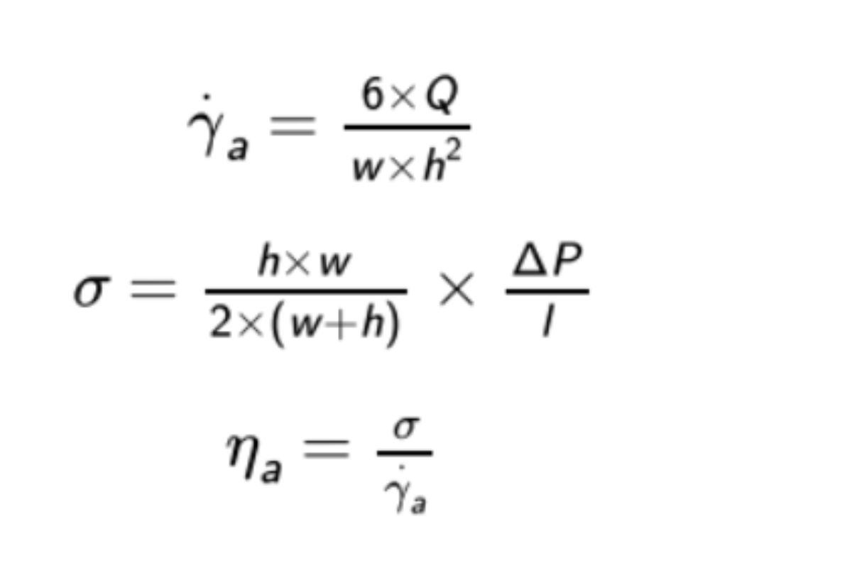
̇γa = apparent shear rate (s−1)
Q = ow rate (µL/s)
w = width of the ow channel (mm)
h = depth of the ow channel (mm)
σ = shear stress (Pa)
ΔP = pressure difference between the leading pressure sensor and the last pressure sensor (Pa) www.webofpharma.com
l = distance between the leading pressure sensor and the last pressure sensor (mm)
ηa = apparent viscosity (Pa · s)
To determine the viscosity of a liquid, pump the liquid sample through the slit channel at a constant flow rate and measure the pressure drop. Using the equations shown above, calculate the apparent viscosity for the apparent shear rate. For a Newtonian liquid, the apparent viscosity is the same as the true viscosity, and the single shear-rate measurement is suficient. For non-Newtonian liquids, the apparent viscosity is not true viscosity. To obtain true viscosity, measure the apparent viscosities at multiple apparent shear rates. Calculate true viscosities, η, at various shear rates using the Weissenberg–Rabinowitsch–Mooney correction factor:
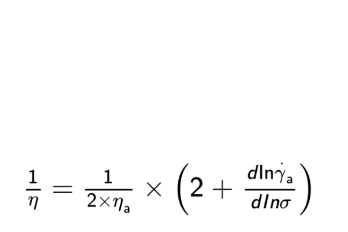
The calculated true viscosity should be the same as the value that is obtained using a cone-and-plate rheometer at the same shear rate.
Procedure: Select slit dimensions and full-scale pressure of pressure sensors to attain the desired range of viscosity and shear rates. With a syringe pump to control the flow rate—or interchangeably, the shear rate—load a test sample into a glass syringe. As necessary, control the temperature of the sample with the syringe and the slit viscometer specified in the individual procedure to ±0.1°, unless otherwise specified. Allow to equilibrate at the specified temperature for about 3–5 min. Set each pressure sensor to zero. Select the first flow rate or shear rate. Pump the sample at the flow rate, and measure the pressure readings once the steady-state values are reached. Increase the
flow rate (or shear rate) until the pressure reading of the leading sensor is >5% of the full-scale value. Take the average of each pressure sensor over time, and calculate the pressure drops. Calculate the apparent viscosity. If required for the procedure, repeat the measurements four times. If the test sample is non-Newtonian, vary the shear rate and calculate the corresponding apparent viscosities.
Calculation and calibration: Calculate the apparent viscosity by dividing the shear stress by the apparent shear rate. For non-Newtonian liquids, apply the Weissenberg–Rabinowitsch–Mooney corrections to obtain the true viscosity curve. Commercial viscometers are provided with a built-in correction.
Calibrate individual pressure sensors by following the recommendations from the manufacturer. The slit viscometer, however, can be calibrated with a Newtonian standard of known viscosity. Choose a standard that covers the viscosity range of interest for the selected slit and pressure sensors. Measure the viscosities at shear rates for 10%, 50%, and 90% of full scale of the leading pressure sensor, and take the average. Calculate a constant (k) for the ratio of the reference value (ηref ) to the measured value (ηmeas ) and record.
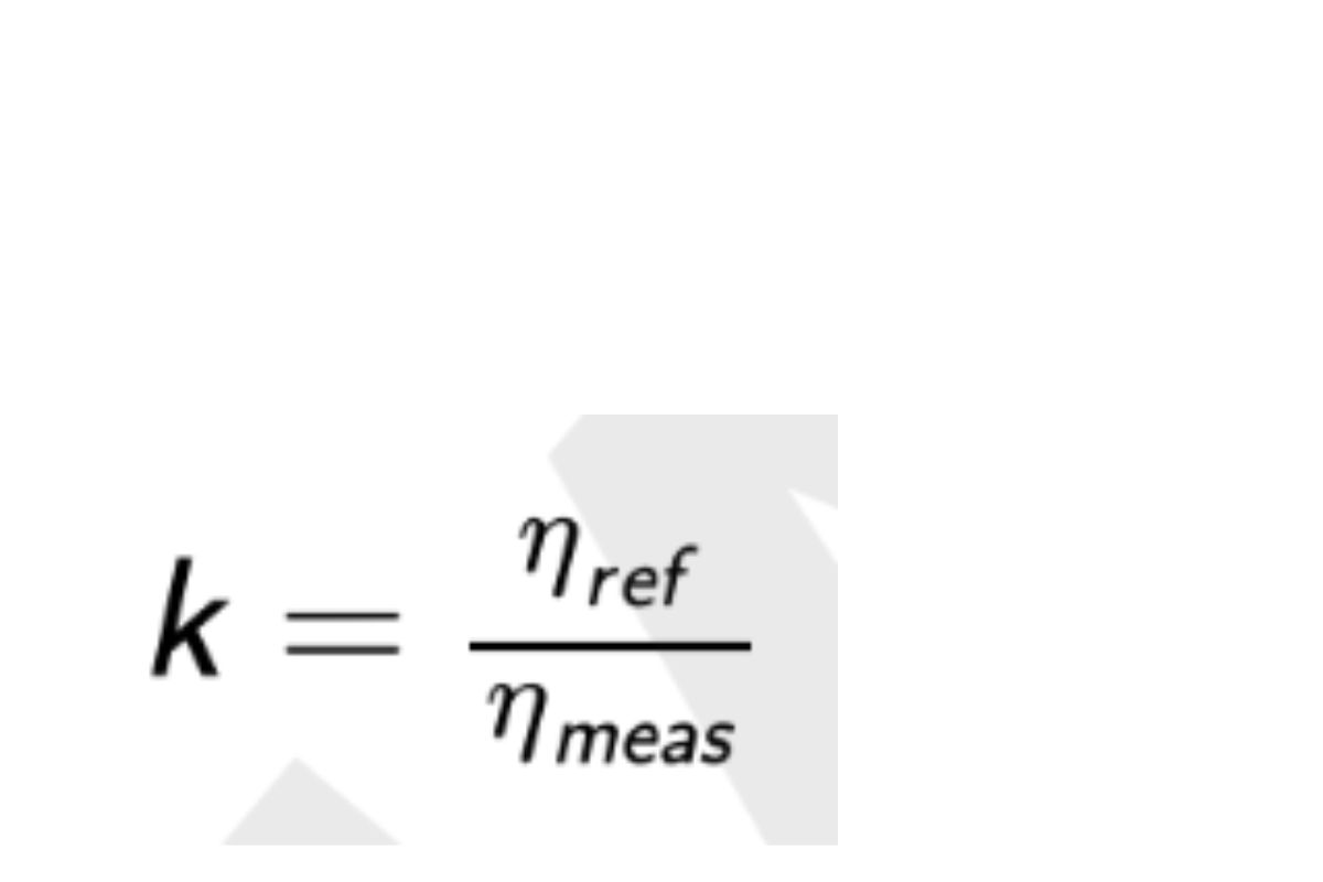
ηref = reference viscosity (Pa · s)
ηmeas = measured viscosity (Pa · s)
Multiply new viscosity data by k, because the value of k will correct for the uncertainty and variation of the slit geometry. Ideally, the value of k should remain constant within a temperature change of 100°. If the k value varies by >1%, consult with the manufacturer regarding the temperature compensation of the pressure sensors.
