Solubility Measurements
If you find any inaccurate information, please let us know by providing your feedback here

Tóm tắt nội dung
- INTRODUCTION
- BACKGROUND
- EXPERIMENTAL METHODS
- METHODS FOR DETERMINATION OF APPARENT SOLUBILITY
- SOLUBILITY MEASUREMENTS IN BIORELEVANT MEDIA (22–26, 30 (USP 1-Aug-2024))
- Human Fasted-State Simulated Gastric Fluid (FaSSGF) (24)
- Human Fed-State Simulated Gastric Fluid (FeSSGF) (24)
- Human Fasted-State Simulated Intestinal Fluid (FaSSIF-V2) (24)
- Human Fed-State Simulated Intestinal Fluid (FeSSIF-V2) (24)
- Human Simulated Colonic Fluid—Proximal Colon (SCoF2) (25)
- Human Simulated Colonic Fluid—Distal Colon (SCoF1) (25)
- Canine Fasted-State Simulated Gastric Fluid (FaSSGFc pH 1.2–2.5) (26)
- Canine Fasted-State Simulated Gastric Fluid (FaSSGFc pH 2.5–6.5) (26)
- Canine Fasted-State Simulated Intestinal Fluid (FaSSIFc) (26)
- Bovine Simulated Ruminal Fluids (27–29)
- Porcine Simulated Gastric and Intestinal Fluids (30)
- Porcine Fasted-State Simulated Gastric Fluid (FaSSGFp) (30)
- Porcine Fasted-State Simulated Intestinal Fluid (FaSSIFp) (30)
- GLOSSARY
- REFERENCES
This article is compiled based on the United States Pharmacopeia (USP) – 2025 Edition
Issued and maintained by the United States Pharmacopeial Convention (USP)
1 INTRODUCTION
[Note—The terms used in this chapter are defined in the Glossary.]
Solutes may differ in both the extent and the rate at which they dissolve in a solvent. Solubility is the capacity of the solvent to dissolve a solute whereas dissolution rate is how quickly the solubility limit is reached. Equilibrium solubility is the concentration limit, at thermodynamic equilibrium, to which a solute may be uniformly dissolved into a solvent when excess solid is present. The apparent solubility may be either higher or lower than the equilibrium solubility due to transient supersaturation or incomplete dissolution due to insufficient time to reach equilibrium. Equilibrium can be defined as sufficiently converged when it no longer changes significantly during a certain time frame. Solubility may be stated in units of concentration such as molality, molarity, mole fraction, mole ratio, weight/volume, or weight/weight.
Solubility can be expressed in absolute as well as relative terms. One method of describing the absolute solubility is the descriptive solubility defined in General Notices, 5.30 Description and Solubility. Relative measures of the solubility are important for predicting the drug delivery characteristics of a dosage form and characterizing a drug as either high solubility or low solubility in the biopharmaceutics classification system (BCS) (1).
Accurate determination of the solubility of pharmaceutical materials is important for understanding both quality control and drug delivery issues for pharmaceutical formulations. The apparent solubility (see the Glossary) of a material is affected by the physicochemical properties of the material (e.g., surface area, particle size, crystal form), the properties of the solubility media (e.g., pH, polarity, surface tension, added surfactants, co-solvents, salts), and the control of the solubility measurement parameters (e.g., temperature, time, agitation method). Additionally, the apparent solubility may be comprised of the intrinsic solubility of the uncharged moiety, the solubility of the ionized compound, and the effect of solubilizers and multiple crystal forms or salt forms. Control of these experimental factors during solubility measurements is key to obtaining accurate, reliable values for the equilibrium solubility of a material.
This chapter will begin with a discussion of the concepts and equations that are relevant to solubility measurements. Understanding these relationships is fundamental to accurate evaluation of solubility. This will be followed by a brief description of typical experimental methods used to assess solubility of pharmaceutical materials. Finally, the use of solubility measurements to obtain biorelevant solubility (for human products) and species-dependent solubility (for veterinary products) will be discussed.
Change to read:
2 BACKGROUND
2.1 Thermodynamic Equilibrium and Solubility
Dissolution of a crystalline solid solute can be modeled by the two-step process of melting the crystal into a pure liquid solute followed by mixing the liquid solute into the solvent. The Gibbs free energy of mixing determines whether, and to what extent, two compounds mix to form a homogeneous phase.
ΔGmix = ΔHmix − TΔSmix
ΔGmix = Gibbs free energy of mixing
ΔHmix = enthalpy of mixing; indicates if the mixing is an endothermic or exothermic process
T = temperature in degrees Kelvin
ΔSmix = change in entropy (disorder) that results from mixing
If the change in the Gibbs free energy is negative, the mixing will be thermodynamically favored. When equilibrium is reached, ΔG will be equal to zero. The enthalpy of mixing is due to the breaking of cohesive interactions (solute–solute, solvent–solvent) and the creation of adhesive interactions (solute–solvent). In other words:
ΔHmix = ΔHUU + ΔHVV − ΔHUV
ΔHmix = enthalpy of mixing
U = solute
V = solvent
This enthalpy change is also equivalent to the work done by removing a volume of pure solvent and a volume of pure solute and exchanging them. The enthalpy change is equal to the newly created interfacial surface energy according to:
γUV = solute–solvent interfacial surface tension
AU= interfacial surface area
γiV = group–solvent interfacial surface tension for group i
Aᵢ = surface area of group i
This equation also shows how the total surface energy can be broken into i smaller groups each with its own surface area, Aᵢ, and corresponding group-water or group-solvent (USP 1-Aug-2024) interfacial tension γᵢV.
For an ideal system, ΔH is zero because the interactions between the ideal solute and ideal solvent are identical. The entropy of mixing for an ideal solution always increases as a result of mixing and is given by:
which under dilute conditions can be simplified to:
For an ideal system under dilute conditions when a crystalline solid is in equilibrium with a saturated solution of the same solute:
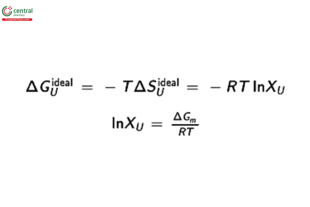
R = gas constant
XU = concentration of the solute expressed as a mole fraction
ΔGm = the free energy change from melting the crystalline solid
Which illustrates how the solubility of the substance can be correlated with the melting point. For a real solution, the solute may also affect (reduce) the disorder in the solvent by inducing structure to the solvent. Therefore, for a real solution, this yields:
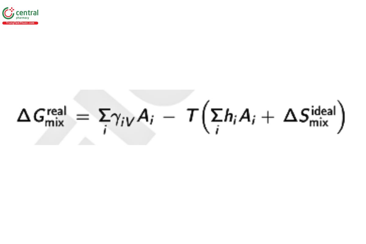
hᵢ = entropic effect on solvent of group i with area Aᵢ
This model allows the total solute surface area (A_U) to be broken into smaller pieces (Σᵢ Aᵢ) and the contribution of these groups to the enthalpic and entropic contributions to the free energy can be estimated.
2.2 Methods of Estimating Aqueous Solubility
Yalkowsky demonstrated (2–3) that a relatively simple general solubility equation (GSE) may be used to empirically estimate the intrinsic solubility of compounds in water.
log S₀ = 0.5 − 0.01(MP − 25) − log KOW
S₀ = intrinsic solubility (of the unionized molecule)
MP = melting point of the crystalline solid (in degrees Celsius)
KOW = octanol–water partition coefficient; the temperature of the water is 25°
The GSE indicates that the aqueous solubility will be reduced for compounds with a higher melting point and compounds with a higher tendency to partition into an oil phase (octanol). The logarithm of the octanol–water partition in the GSE accounts for the difference between an ideal solution and an aqueous solution due to the enthalpy of mixing (3). The GSE can also be used to predict the solubility of ionizable compounds by combining it with the Henderson–Hasselbalch equation if the pKₐ is known (see Effect of pH).
Use of GSE requires the measurement of the melting point and partition coefficient (and pKₐ for ionizable compounds). There are several computer programs that will support the estimation of the partition coefficient and the pKₐ for compounds based on structure (4), but this is not the case for melting points. Efforts to develop computational methods to predict aqueous solubilities have relied on training sets of molecules to search for correlations with properties that can be more easily predicted from the structure (e.g., molecular weight, solvent-accessible surface area, number of rotatable bonds, etc.) (5). The success of these computational approaches is often limited to molecules that are similar to the training set. These calculational methods are adequate for providing assistance in prescreening synthetic candidates, but are not sufficiently accurate to substitute for experimental solubility.
2.3 Factors that Affect Solubility and Solubility Measurements
2.3.1 Effect of pH
The solubility of ionizable acids and bases is pH-dependent because the charged species have a higher affinity for the aqueous environment than the neutral form. The total solubility of the ionizable acid or base is the sum of the intrinsic solubility and the amount of ionized solute present at that pH. The Henderson–Hasselbalch equation relates the increase in the solubility to the pH of the solution relative to the pKₐ (acidic) or pKb(USP 1-Aug-2024) (basic) of the ionizable acid or base.
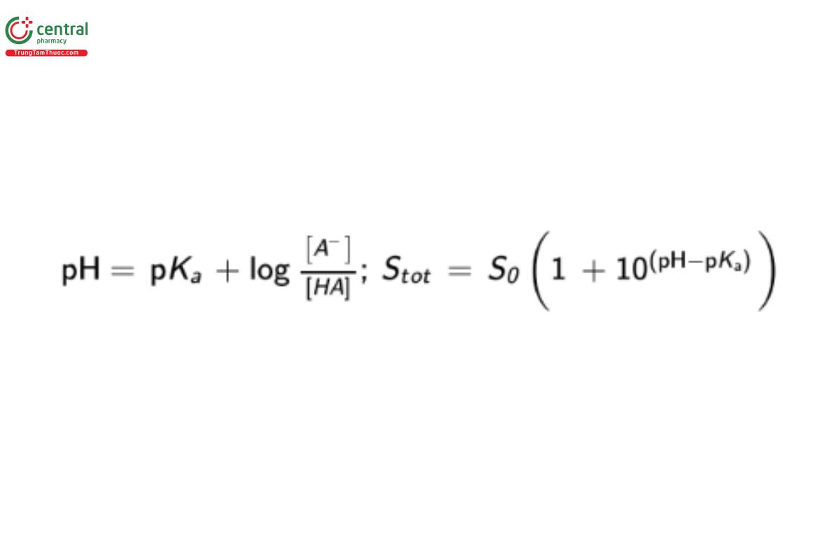
pKₐ = −log(Kₐ)
Kₐ = acid dissociation constant
[A⁻] = molar concentration of the acid’s conjugate base
[HA] = molar concentration of the undissociated weak acid
Stot = total solubility of weak acid
S₀ = intrinsic solubility of uncharged moiety
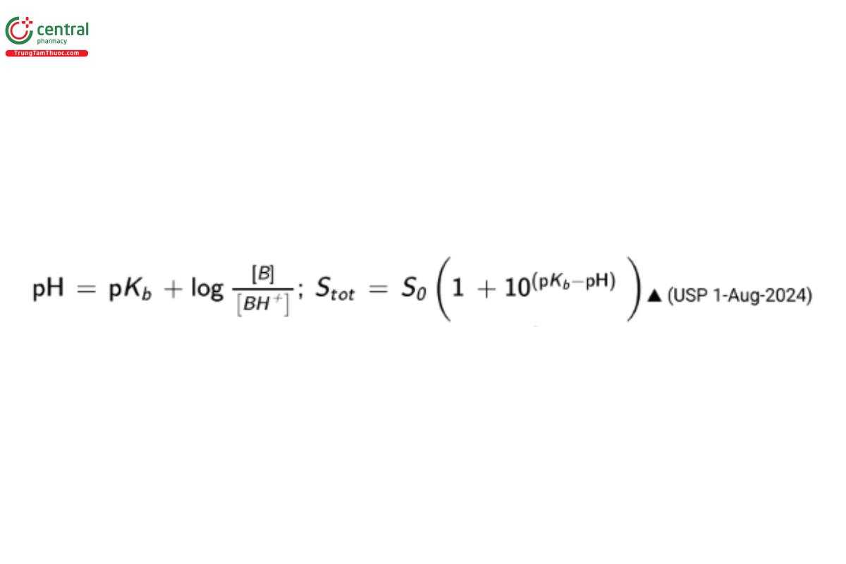
pKb(USP 1-Aug-2024) = −log(Kb)
Kb(USP 1-Aug-2024) = base dissociation constant
[B] = molar concentration of the base’s conjugate base
[BH⁺] = molar concentration of the dissociated base
Stot = total solubility of weak base
S₀ = intrinsic solubility of uncharged moiety
The Henderson-Hasselbalch equation helps explain the increase in solubility at the first pKₐ, but is not useful for modeling the behavior of polyprotic acids over a pH range incorporating additional pKₐ values. Because ionizable molecules can differ in the number and type of ionizable groups, it is important to explore solubility across a range of pH values. Figure 1 illustrates this pH dependence of the solubility for a molecule with two ionization constants of 5.6 and 11.7. The molecule is charged below pH 5.6 and above 11.7 and is neutral between these two pH values. Where the molecule is unionized, the solubility is equal to the intrinsic solubility. For the ionized molecule, the solubility increases on a log scale as the pH changes. The formation of a salt may limit the solubility at a low or high pH (see Figure 1). If the acid used to adjust the pH contributes the counter-ion for the salt, the common-ion effect will further suppress the solubility as the counter-ion concentration is increased (see Figure 1). If the salt is dissolved at higher pH, the salt may supersaturate the solution initially, but will eventually precipitate as whatever solid form has lower solubility at that pH (6).
Figure 1. Effect of pH on solubility for an ionizable compound. When the molecule is unionized, the solubility is equal to the intrinsic solubility. For the ionized molecule, the solubility increases on a log scale as the pH changes. The salt solubility limits the solubility at a low pH. If the acid used to adjust the pH contributes the counter-ion for the salt, the common-ion effect will further suppress the solubility as the counter-ion concentration is increased (apparent at pH <2 in the figure).
2.3.2 Effect of salts and counter-ions
Ionizable compounds can also form salts with an oppositely charged counter-ion (6). In a solution, in the presence of the charged counter-ion, the solubility product describes this equilibrium reaction as follows:
For the salt dissolution, AₙBₘ(s) → nA⁺(aq) + mB⁻(aq)
solubility product, Ksp = [A⁺]ⁿ[B⁻]ᵐ
The maximum solubility of the salt in a solution is also illustrated in Figure 1. As a result of the formation of the salt, the actual solubility of the charged molecule is seen to plateau (at a pH below the pKₐ of the drug in this example) instead of continuing to increase as predicted by the Henderson–Hasselbalch equation. Because the solubility product, Ksp, is a constant, the solubility of the ionizable moiety may drop even further if the acid being used to adjust the pH increases the concentration of the oppositely charged counter-ion. The reduction in the solubility of the charged molecule as the counter-ion concentration is increased is referred to as the common-ion effect (6). This is frequently seen when hydrochloric acid (HCl) is used to reduce the pH, and the solubility of the chloride salt is reduced due to increasing chloride concentration (e.g., at pH <2). Although not illustrated in Figure 1, salts may also limit the solubility on the basic side of the plot (e.g., a sodium salt of an acid moiety), and the common-ion effect may similarly affect the solubility at a high pH when the compound used to adjust the pH has a common-ion (e.g., sodium hydroxide).
2.3.3 Effect of co-solvents
Water is often a poor solvent for many pharmaceutical ingredients, but water is miscible with other solvents that may provide good solubility for these substances (e.g., Ethanol, propylene glycol, polyethylene glycol, etc.). According to the log-linear model (2), the log S of the solute can generally be linearly interpolated between two miscible co-solvents. This relationship is illustrated in Figure 2. When this solubility plot is switched to a linear scale, it becomes evident that even low concentrations of the poor solvent (typically water) in the co-solvent mixture can dramatically reduce the solubility for the solute. For this reason, solutions containing co-solvents are particularly prone to precipitation when diluted due to the significant change in solubility. [Note—This simple model, as depicted in Figure 2, assumes that maximum solubility occurs at 100% of the good solvent and this may not be the case for all co-solvent systems.]
Figure 2. Illustration of the log-linear model of Yalkowsky and co-workers (2). The log of solubility appears to be linear as a function of the co-solvent fraction. When plotted on a linear scale, it is apparent that the solubility drops exponentially as the poor solvent is added to the better solvent.
2.3.4 Effect of surfactants
Surfactants are amphiphiles, which are characterized by polar and nonpolar regions. When placed in water, a surfactant prefers to reside at the air-water interface and orients its polar region in water and its nonpolar region to the less polar interface (air). When the air-water interface is saturated with adsorbed surfactant, additional surfactant molecules aggregate into a spherical micelle with a polar surface and a nonpolar core. This point when micelles form is known as the critical micelle concentration (CMC). Above the CMC, the number of micelles in a solution increases linearly as the concentration of surfactant increases. If a pharmaceutical material is able to partition into the micelle, its solubility will increase linearly as the number of micelles increases (see Figure 3). The CMC for surfactants is dependent on several factors including temperature, ionic strength, and pH. As an example, the CMC for sodium lauryl sulfate is 6 mM, and the CMC for Polysorbate 80 is 0.012 mM, in pure water at 25°. The solubilization of a molecule by a surfactant can be evaluated based on two descriptors: the molar solubilization capacity, and the micelle-water partition coefficient. The micelle-water partition coefficient is the ratio of drug concentration in the micelle to the drug concentration in water for a particular surfactant concentration (7).
Figure 3. Solubility enhancement by surfactants. Solubilization requires the formulation of micelles. Below the CMC, added surfactant results in monomers of surfactant dissolved in the solvent and no solubility enhancement occurs. Above the CMC, the solubility increases linearly. The slope of this linear increase indicates the solubilization capacity of the micelles.
As illustrated in Figure 3, the solubility in the presence of surfactants is the additive combination of the amount dissolved in the aqueous phase plus the amount solubilized by the micelles. The micelles will be larger than the solute and will diffuse more slowly than the solute. Drug delivery in the presence of micelles will be due to the absorption of the free drug in solution as well as drug delivery by micelle-mediated transport (5–6). Therefore, solubilization by surfactants may not result in an enhancement in drug delivery that is directly proportional to the increase in aqueous solubility (5–6).
2.3.5 Effect of complexing agents
Complexing agents may form intermolecular complexes with low-solubility materials and enhance the solubility. Aqueous solubility of nonpolar molecules in the presence of complexing agents is improved as the nonpolar molecules and the nonpolar region of the complexing agent are sequestered out of water. When this occurs, the aqueous solution can accommodate more of the nonpolar molecules. Regardless of the ratio of ligand to solute in these complexes (e.g., 1:1, 2:1, 3:1, etc.), the solubility enhancement is expected to increase as the concentration of the complexing agent increases (8). This is very similar to solubilization by surfactants except there will not be a minimum concentration of the complexing agent required. Complexes with high stability constants may bind solutes strongly enough to enhance aqueous stability. Cyclodextrins are often used to enhance solubility by forming complexes with drug substances.
2.3.6 Effect of surface area (dissolution rate)
The Noyes–Whitney equation (as expressed by Nernst and Brunner) states:
Rate = ∂C/∂t = DA(CS − C)/h
C = concentration of the solute in the solvent at time, t
D = diffusivity of the solute
A = surface area of the solute particles
CS = saturated solubility of the solute
h = thickness of the diffusion layer
In unstirred solutions, the diffusion layer thickness, h, may be large and is primarily affected by the diffusivity of the solute; however, good mixing may significantly reduce the diffusion layer thickness. For small particles in well-mixed solutions, the diffusion layer thickness, h, was found (9) to be proportional to the square root of the particle radius. This equation indicates that the smaller particles will have greater surface area and will dissolve more quickly. In order to reach the equilibrium solubility as quickly as possible, the surface area should be kept as high as possible (i.e., smaller particles) and the diffusion layer thickness kept as small as possible (i.e., good mixing) (9).
For spherical particles, the surface area, A, can be expressed as a function of the total mass, M:
A = 6M/ρd
For spherical particles:
ρ = density
d = particle diameter
Rate = ∂C/∂t = (6DM/ρdh)(CS − C)
The dissolution rate of a material will not affect the equilibrium solubility, but will affect how quickly this equilibrium is achieved.
2.3.7 Effect of surface energy
The surface energy of the particle may affect the solubility. According to the Kelvin equation, smaller particles have higher solubility than larger particles due to the effect of the surface energy on the total Gibbs free energy of the system. Typically, this effect on solubility only becomes significant for particles smaller than 1 micron. The Kelvin equation quantifies this as:
ln(S/S₀) = 4γVm/(RTd)
S = apparent solubility
S₀ = solubility of an infinitely large particle
γ = surface energy of the solute
Vm = molecular volume of the solute
R = gas constant
T = temperature
d = diameter of the particle
The solubility difference between smaller and larger particles leads to so-called Ostwald ripening in polydisperse suspensions. The small particles dissolve and result in a solution that is supersaturated relative to the solubility of the larger particles. This leads to recrystallization on the surface of the larger particles. The larger particles grow in size while the smaller particles dissolve resulting in an increase in the mean particle size of the suspension (10).
Change to read:
3 EXPERIMENTAL METHODS
3.1 Methods for Determination of Equilibrium Solubility
3.1.1 Saturation shake-flask method
The shake-flask method is based on the phase solubility technique that was developed 40 years ago and is still considered by most to be the most reliable and widely used method for solubility measurement today (11–18). The shake-flask method should be used when equilibrium solubility needs to be determined. Other methods may be used to evaluate apparent solubility, but are not considered suitable for evaluation of true equilibrium solubility.
The solubility medium selected for solubility measurements should be selected to be relevant to the application with efforts made to control the surfactant type and concentration, the ionic strength of the buffer, and the types of counter-ions present in the buffer. When the results are intended to predict absorption or bioavailability, it is recommended that one of the biorelevant media solutions be used (see Solubility Measurements in Biorelevant Media). When the results are intended to support the development of dissolution tests, it is recommended that the dissolution medium be used. For research purposes, when the pH dependence of the compound is being evaluated, a buffer that allows control of ionic strength and counter-ion types over a wide pH range is recommended (e.g., Britton–Robinson or Sörensen buffers). For solubility measurements that will be used for BCS classification, USP-recommended buffers should be used unless otherwise justified (USP 1-Aug-2024) (19).
Sample preparation: The test substance is typically prepared by adding an excess of solid to the solubility medium, which is in a stoppered flask or vial. The amount of medium in the flask or vial does not need to be measured accurately. It is mandatory (USP 1-Aug-2024) that the solid be added to the solubility medium in an amount that ensures saturation (USP 1-Aug-2024). The surface area of the solid may be increased by grinding (e.g., in a mortar and pestle) of the sample prior to addition to the medium or by sonication of the sample after addition to the medium. [Caution—It is advised to use caution when employing high-energy methods to increase the surface area because it may alter the solid form of the solute.] It is recommended that sample preparation be performed in triplicate to provide at least 3 solubility results for each test condition.
Equilibration of solution: To facilitate dissolution of the solid, the suspension should be actively mixed or agitated. As a good initial time of incubation, 24 h is recommended; however, the suitability of the selected equilibration time must be verified. The temperature of the suspension should be well controlled during this dissolution phase (±0.5°). Following the dissolution phase, it is recommended that the excess solid be allowed to sediment completely. Sedimentation and decantation are recommended as the safest method for separation of the solid from the saturated solution. For non-clarifying colloid solutions, centrifugation can be used. Sampling of the supernatant should avoid incorporating any undissolved solid, as this will significantly affect the solubility result. The transfer pipet needs to be pretreated with sample solution before use, so that surface adsorption is not altering the transferred solution. If filtration cannot be avoided, then it is essential that the proper filter type is selected. For polar, ionized species, hydrophobic type filters (nylon) are recommended; while for unionized species the hydrophilic type filters [e.g., polyvinylidene difluoride (PVDF) or polyethersulfone (PES)] are recommended. The filtration should be done after sedimentation, and not directly after agitation. Presaturation of the filter is necessary (i.e., the initial portions of filtrate should be discarded). The temperature of the suspension during the sedimentation and centrifugation steps must also be well controlled (±0.5°) and be equivalent to the temperature at which solubilization occurred.
Saturation (equilibrium) has been reached when multiple samples, assayed after different equilibration time periods, yield equivalent results (e.g., change by less than 5% over 24 h, or less than 0.2%/h). To confirm that the apparent solubility is the equilibrium solubility, it is recommended that the same suspension be re-equilibrated via the same procedure (e.g., mix for an additional 24 h).
Analysis of solution: The requirements for the analytical method used to quantitate the concentration of the solute and the level of analytical validation required should be commensurate with the intended use of the solubility data. In general, the method should be linear and specific. The supernatant solution may need to be diluted before analysis to be within the linearity of the analytical method and to avoid possible precipitation. The solution may be analyzed by UV-Vis spectrometry or by liquid chromatography methods to determine the soluble concentration. The advantage of HPLC is that it can detect instability by resolving drug-related impurities (13,20).
It is recommended that the excess solid in the suspension be analyzed at the end of the solubility measurement to verify that the solid form has not changed. In cases where the solid form has changed, it is likely that the new solid form has a lower solubility than the initial solid form and that the observed solubility is due to the new lower-solubility form; however, this should be evaluated on a case-by-case basis. Powder X-ray diffraction (PXRD), Raman or near-infrared (NIR) spectrometry, or evaluation of the melting point by differential scanning calorimetry (DSC) are examples of techniques that can be used to evaluate the solid form. Solutes that are unstable (either chemically or physically) during the equilibration time are not suitable for equilibrium solubility measurements by the shake-flask method. For example, amorphous drugs that will convert to lower solubility salts or polymorphs should be analyzed using one of the apparent solubility methods.
Reporting of solubility results: If a non-standard composition for the media is used in the solubility determination, the details of the composition should be reported. The ionic strength of the media used in the solubility determination should be calculated and reported with the solubility result. The pH of the supernatant solution should be recorded (at the temperature of the solubility measurement) when the sample is withdrawn for analysis. When using well-defined, standard media, it is recommended that the pH of the media not be adjusted to compensate for alteration of the pH by the dissolving species; rather, the solubility value should be reported at the pH value and temperature observed at the end of the equilibration step (12.18). If the pH of the media is significantly affected by the dissolving species and solubility at a particular pH is desirable, it is recommended to perform an additional solubility measurement in a higher buffer-capacity medium. Report the mean temperature and the precision of temperature control during the equilibration.
The precision of the reported equilibrium solubility should reflect the level of agreement between the measurements rather than the precision of the solubility analysis. Standard deviations in the measured solubility (based on averaging 3 or more independent samples) should be included.
4 METHODS FOR DETERMINATION OF APPARENT SOLUBILITY
4.1 Intrinsic Determination (Rotating Disk)
The measurement of intrinsic dissolution is described more fully in Intrinsic Dissolution—Dissolution Testing Procedures for Rotating Disk and Stationary Disk 〈1087〉. This measurement technique may also be used to assess the solubility.
To apply this method to the measurement of solubility, the dissolution experiment must be continued to the point that the rate of dissolution is insignificant (e.g., less than 5%/24 h or less than 0.2%/h).
All the requirements discussed for the shake-flask method in Analysis of solution and Reporting of solubility results will also apply to measurements using the intrinsic dissolution apparatus.
4.2 Potentiometric Titration
The potentiometric acid–base titration for solubility measurements is based on a characteristic shift in the middle of the titration curve that is caused by precipitation (21). For the titration, accurate volumes of a standardized acid or base are added to a solution containing an ionizable substance and a salt, for example, 0.15 M potassium chloride (KCl), which is included to increase the accuracy of the measurements.
Sparging (a technique that involves bubbling a chemically inert gas such as nitrogen, argon, or helium through a liquid) with argon prevents carbon dioxide (CO₂) from the atmosphere from influencing the pH value.
A glass electrode is used to monitor the pH value continuously. The potentiometric titration curve is obtained by plotting the pH value against the consumed volume of acid/base (21).
4.3 Turbidimetry
Turbidimetry involves the dissolution of a compound in an organic solvent, for example, Dimethyl sulfoxide (DMSO). The resulting solution is added to a buffer solution in intervals adequate to characterize changes in turbidity. Further aliquots of the solution are added after the first detection of turbidity by light scattering. Subsequently, the volume added can be plotted against the turbidity. The solubility is then estimated by back-extrapolation to the point where precipitation began. This method can be used to measure as many as 50–300 samples per day. When using solvents such as DMSO, drawbacks include the increase in solubility of the drug substance for the short duration of the experiment, which leads to a kinetic rather than thermodynamic solubility, the formation of a supersaturated solution, and the undefined crystalline form of the precipitated solid (unless it is removed from the suspension and characterized).
4.4 Physical Assessment of Solubility
For compounds with extremely high solubility, as well as for biologics and other molecules that lack chromophores or are not easy to quantitate in solution, a physical assessment of solubility may be used to assess apparent solubility. In this case, the principle of measurement is the loss of solid material to the solution phase. Equilibrium may be assessed by both the stability of the weight loss as well as the stability of the change in the physical properties of the resulting solution (e.g., refractive index, density, osmolality, etc.). Because the physical assessment of solubility does not involve a specific or stability-indicating assay, it is recommended that some attempt be made to verify the stability and purity of the solute. Also, evaporation of the solvent should be carefully monitored and controlled during the solubility measurement performed by this method.
Change to read:
5 SOLUBILITY MEASUREMENTS IN BIORELEVANT MEDIA (22–26, 30 (USP 1-Aug-2024))
The use of simple aqueous buffers to evaluate the aqueous solubility of a drug substance as a function of pH may underestimate the bioavailability (22–23). The media recipes presented here are examples that may be used to evaluate the solubility in simulated human, canine, bovine (ruminant), and porcine (USP 1-Aug-2024) fluids to make improved estimates of bioavailability.
The temperature of the solubility medium should be controlled at ±0.5° during biorelevant solubility measurements. Biorelevant solubility measurements should follow the shake-flask method, including solubility measurements at multiple time points to confirm that equilibrium has been achieved. The salt form of a drug added to the solubility medium may significantly affect the composition of the medium (i.e., ionic strength, pH, etc.). Therefore, the solubility of a salt and a free base of the same drug should not be assumed to be equivalent unless proven through independent measurements starting with the different crystalline solids.
6 Human Fasted-State Simulated Gastric Fluid (FaSSGF) (24)
The pH is 1.6 at 37°. See Table 1 for the media composition.
Table 1
| Ingredient | Concentration (mM) | Concentration (g/L) |
| Hydrochloric acid | ~31.3 (q.s. to pH 1.6) | ~1.14 (q.s. to pH 1.6) |
| Sodium chloride | 34.2 | 2.00 |
| Sodium taurocholate | 0.08 | 0.043 (USP 1-Aug-2024) |
| Lecithin | 0.02 | 0.013 (USP 1-Aug-2024) |
| Pepsin | — | 0.1 |
6.1 Human Fed-State Simulated Gastric Fluid (FeSSGF) (24)
The pH is 5 at 37°. See Table 2 for the media composition.
Table 2
| Ingredient | Concentration (mM) | Concentration (g/L) |
| Hydrochloric acid | (q.s. to pH 5) | (q.s. to pH 5) |
| Sodium hydroxide | (q.s. to pH 5) | (q.s. to pH 5) |
| Sodium chloride | 237.0 | 13.85 |
| Sodium acetate | 29.75 | 2.440 (USP 1-Aug-2024) |
| Acetic acid | 17.12 | 1.028 |
| Milk, whole | 1:1 | 1:1 |
6.2 Human Fasted-State Simulated Intestinal Fluid (FaSSIF-V2) (24)
The pH is 6.5 at 37°. See Table 3 for the media composition.
Table 3
| Ingredient | Concentration (mM) | Concentration (g/L) |
| Maleic acid | 19.12 | 2.219 |
| Sodium hydroxide | 34.8 | 1.392 |
| Sodium chloride | 68.62 | 4.010 |
| Sodium taurocholate | 3.0 | 1.613 (USP 1-Aug-2024) |
| Lecithin | 0.2 | 0.129 (USP 1-Aug-2024) |
6.3 Human Fed-State Simulated Intestinal Fluid (FeSSIF-V2) (24)
The pH is 5.8 at 37°. See Table 4 for the media composition.
Table 4
| Ingredient | Concentration (mM) | Concentration (g/L) |
| Maleic acid | 55.02 | 6.386 (USP 1-Aug-2024) |
| Sodium hydroxide | 81.65 | 3.266 (USP 1-Aug-2024) |
| Sodium chloride | 125.5 | 7.334 (USP 1-Aug-2024) |
| Sodium taurocholate | 10 | 5.377 (USP 1-Aug-2024) |
| Lecithin | 2.0 | 1.29 (USP 1-Aug-2024) |
| Glyceryl monostearate | 5.0 | 1.793 (USP 1-Aug-2024) |
| Sodium oleate | 0.8 | 0.244 (USP 1-Aug-2024) |
6.4 Human Simulated Colonic Fluid—Proximal Colon (SCoF2) (25)
The pH is 5.8 at 37°. See Table 5 for the media composition.
Table 5
| Ingredient | Concentration (mM) | Concentration (g/L) |
| Sodium hydroxide | ~157 (q.s. to pH 5.8) | ~6.28 (q.s. to pH 5.8) |
| Acetic acid, glacial | 170 | 10.209 (USP 1-Aug-2024) |
6.5 Human Simulated Colonic Fluid—Distal Colon (SCoF1) (25)
The pH is 7.0 at 37°. See Table 6 for the media composition.
Table 6
| Ingredient | Concentration (mM) | Concentration (g/L) |
| Potassium chloride | 2.68 (USP 1-Aug-2024) | 0.20 (USP 1-Aug-2024) |
| Sodium chloride | 136.89 (USP 1-Aug-2024) | 8.00 (USP 1-Aug-2024) |
| Potassium phosphate, monobasic | 1.76 (USP 1-Aug-2024) | 0.24 |
| Sodium phosphate, dibasic | 10.14 (USP 1-Aug-2024) | 1.44 |
6.6 Canine Fasted-State Simulated Gastric Fluid (FaSSGFc pH 1.2–2.5) (26)
Canine gastric pH can vary substantially. Due to interstudy variations in the canine gastric pH estimates, solubility should be evaluated over a range of 1.2–6.5. The pH of this fluid is adjusted by altering the amount of hydrochloric acid so that pH values in the range of 1.2–2.5 may be achieved.
The pH is 1.2–2.5 at 37°. See Table 7 for the media composition.
Table 7
| Ingredient | Concentration (mM) | Concentration (g/L) |
| Hydrochloric acid | ~3.6–82 (q.s. to pH 1.2–2.5) | ~0.13–3 (q.s. to pH 1.2–2.5) |
| Sodium chloride | 14.5 | 0.8474 (USP 1-Aug-2024) |
| Sodium taurocholate | 0.10 | 0.0538 (USP 1-Aug-2024) |
| Sodium taurodeoxycholate | 0.10 | 0.0522 (USP 1-Aug-2024) |
| Lecithin | 0.025 | 0.0161 (USP 1-Aug-2024) |
| Lysolecithin | 0.025 | 0.0124 (USP 1-Aug-2024) |
| Sodium oleate | 0.025 | 0.0076 |
6.7 Canine Fasted-State Simulated Gastric Fluid (FaSSGFc pH 2.5–6.5) (26)
Canine gastric pH can vary substantially. Due to interstudy variations in the canine gastric pH estimates, solubility should be evaluated over a range of 1.2–6.5. The pH of this fluid is adjusted by altering the amount of sodium hydroxide so that pH values in the range of 2.5–6.5 may be achieved. The pH is 2.5–6.5 at 37°. See Table 8 for the media composition.
Table 8
| Ingredient | Concentration (mM) | Concentration (g/L) |
| Maleic acid | 21.68 | 2.5164 (USP 1-Aug-2024) |
| Sodium hydroxide | ~14.5–40 (q.s. to pH 2.5–6.5) | ~0.58–1.6 (q.s. to pH 2.5–6.5) |
| Sodium chloride | 18.81 | 1.0993 (USP 1-Aug-2024) |
| Sodium taurocholate | 0.10 | 0.0538 (USP 1-Aug-2024) |
| Sodium taurodeoxycholate | 0.10 | 0.0522 (USP 1-Aug-2024) |
| Lecithin | 0.025 | 0.0161 (USP 1-Aug-2024) |
| Lysolecithin | 0.025 | 0.0124 (USP 1-Aug-2024) |
| Sodium oleate | 0.025 | 0.0076 |
6.8 Canine Fasted-State Simulated Intestinal Fluid (FaSSIFc) (26)
The pH is 7.5 at 37°. See Table 9 for the media composition.
Table 9
| Ingredient | Concentration (mM) | Concentration (g/L) |
| Sodium dihydrogen phosphate, monohydrate | 28.65 | 3.953 (USP 1-Aug-2024) |
| Sodium hydroxide | 21.66 | 0.8664 (USP 1-Aug-2024) |
| Sodium chloride | 59.63 | 3.4848 (USP 1-Aug-2024) |
| Sodium taurocholate | 5.0 | 2.69 (USP 1-Aug-2024) |
| Sodium taurodeoxycholate | 5.0 | 2.6085 (USP 1-Aug-2024) |
| Lecithin | 1.25 | 0.8048 (USP 1-Aug-2024) |
| Lysolecithin | 1.25 | 0.6195 (USP 1-Aug-2024) |
| Sodium oleate | 1.25 | 0.3806 (USP 1-Aug-2024) |
6.9 Bovine Simulated Ruminal Fluids (27–29)
The media defined here are suitable to represent bovine as well as other ruminant species. The normal pH of a healthy reticulo-rumen is in the 5.5–6.8 range. High-grain diets typically result in a lower ruminal pH (~5.5), whereas high-forage diets result in a higher ruminal pH (~6.8).
In the abomasum (true stomach), the pH is about 2–3 and is similar to conditions observed in monogastrics and humans. To represent the abomasum, one may use 0.01 M hydrochloric acid (pH 2), 0.0033 M hydrochloric acid (pH 2.5), or 0.001 M hydrochloric acid (pH 3). Intestinal pH in ruminants is similar to that observed in monogastrics and humans. The pH at the pylorus is about 3.0 and increases to about 7.5 in the ileum. To represent the bovine intestinal fluids, one may use one of the simulated intestinal fluids defined for human or canine above.
The temperature is set for 39°. [Note—The pH of media should be confirmed at 39°.] See Table 10 for the media composition.
Table 10
| Ingredient | High-Grain Diet Simulated Rumen | High-Forage Diet Simulated Rumen |
| Tryptone | 2.5 g/L | 2.5 g/L |
| Sodium bicarbonate | 3.999 g/L (47.6 mM) (USP 1-Aug-2024) | 8.737 g/L (104 mM) (USP 1-Aug-2024) |
| Potassium phosphate monobasic anhydrous | 1.55 g/L (11.4 mM) | 1.55 g/L (11.4 mM) |
| Sodium phosphate dibasic anhydrous | 1.420 g/L (10.0 mM) (USP 1-Aug-2024) | 1.420 g/L (10.0 mM) (USP 1-Aug-2024) |
| Ammonium bicarbonate | 0.996 g/L (12.6 mM) (USP 1-Aug-2024) | 0.996 g/L (12.6 mM) (USP 1-Aug-2024) |
| Magnesium sulfate heptahydrate | 0.148 g/L (0.6 mM) (USP 1-Aug-2024) | 0.148 g/L (0.6 mM) (USP 1-Aug-2024) |
| Acetic acid | 2.402 g/L (40 mM) (USP 1-Aug-2024) | 1.441 g/L (24 mM) (USP 1-Aug-2024) |
| Propionic acid | 2.593 g/L (35 mM) (USP 1-Aug-2024) | — |
| Butyric acid | 1.322 g/L (15 mM) (USP 1-Aug-2024) | — |
| Sodium acetate trihydrate | — | 6.26 g/L (46 mM) |
| Sodium propionate | — | 1.44 g/L (15 mM) |
| Sodium butyrate | — | 1.10 g/L (10 mM) |
| Micromineral stock solution (see Table 11) | 125 µL | 125 µL |
| pH | 5.5 | 6.8 |
| Surface tension | ~50 dynes/cm² | ~50 dynes/cm² |
| Ionic strength | 0.102 mol/L | 0.240 mol/L |
| Buffer capacity | 47 mmol/L/pH | 49 mmol/L/pH |
Table 11
| Ingredient | Concentration (g/L(USP 1-Aug-2024)) |
| Water | q.s. to 1 L (USP 1-Aug-2024) |
| Calcium chloride dihydrate | 132.0 (USP 1-Aug-2024) |
| Manganese chloride tetrahydrate | 100.0 (USP 1-Aug-2024) |
| Iron (III) chloride hexahydrate | 80.0 (USP 1-Aug-2024) |
6.10 Porcine Simulated Gastric and Intestinal Fluids (30)
The porcine simulated gastric and intestinal fluids reflect information reported by Henze et al. (30), based upon their analysis of the gastrointestinal fluid content of fasted landrace pigs.
6.11 Porcine Fasted-State Simulated Gastric Fluid (FaSSGFp) (30)
The gastric pH of fasted landrace pigs varies from 1.7–3.4, with a mean value of 2.2 ± 0.7. Other physicochemical properties such as buffer capacity (6.1 ± 3.5 mmol/L for pigs, 14.3 ± 9.3 mmol/L for humans) and surface tension (46.5 ± 1.3 mN/m for pigs, 31–45 mN/m for humans) were similar to that of human FaSSGF. Swine-human differences were observed in fasted gastric osmolality (99 ± 53 mOsm/kg for pigs, 220 ± 58 mOsm/kg for humans).
In general, given the similarity in the composition of porcine and human fasted gastric fluids, the use of human FaSSGF, adjusted to pH 2.2 at 39°, is recommended for testing drug solubility in swine.
6.12 Porcine Fasted-State Simulated Intestinal Fluid (FaSSIFp) (30)
The pH is 7.0 at 39°. See Table 12 for the media composition.
Table 12
| Ingredient | Concentration (mM) | Concentration (g/L) |
| Sodium phosphate monobasic, anhydrous | 35.71 | 4.284 |
| Sodium hydroxide | 13.62 | 0.545 |
| Sodium chloride | 135.32 | 7.908 |
| Sodium taurodeoxycholate | 9.72 | 5.071 |
| Sodium taurocholate | 5.25 | 2.823 |
| Sodium oleate | 2.82 | 0.859 |
| Lecithin | 0.20 | 0.129 |
(USP 1-Aug-2024)
7 GLOSSARY
[Note—The following definitions are provided to clarify the use of these terms in the context of this chapter. These definitions are not intended to supersede or contradict definitions found elsewhere in the USP–NF.]
Apparent solubility: The empirically determined solubility of a solute in a solvent system where insufficient time is allowed for the system to approach equilibrium or where equilibrium cannot be verified. The apparent solubility may be either higher or lower than the equilibrium solubility due to transient supersaturation or incomplete dissolution and insufficient time to reach equilibrium.
Aqueous solubility: Solubility in a medium that is primarily comprised of water but may also contain solubilization enhancement from co-solvents, surfactants, complexing agents, pH, or other co-solutes. The term “aqueous solubility” is very general and should not be confused with water solubility. Aqueous solubility is significantly affected by the composition of the aqueous medium.
Dissolution: The non-equilibrium process of approaching the solubility limit at thermodynamic equilibrium (i.e., the solute and solvent forming a uniformly mixed solution). The dissolution rate will affect the time required to reach equilibrium and may affect the apparent solubility, but will not affect the final equilibrium solubility.
Equilibrium solubility: The concentration limit, at thermodynamic equilibrium, that a solute can dissolve into a saturated solution when excess solid is present. Equilibrium can be defined as sufficiently converged when it no longer changes significantly during a certain time frame.
Intrinsic solubility: The solubility of the uncharged (neutral) moiety. Intrinsic solubility can only be accurately measured in pH ranges where the distribution of species is dominated by the uncharged molecule. For some compounds, it may be impossible to directly measure the intrinsic solubility and it must be determined by fitting the solubility data as a function of pH.
Solubility: The extent to which a solute may be uniformly dissolved into a solvent. This may be referred to as equilibrium (saturated) solubility to differentiate it from apparent solubility. Solubility may be stated in units of concentration such as molality, mole fraction, mole ratio, weight/volume, and weight/weight.
Water solubility: Solubility in pure water. Measurements of solubility in pure water are problematic due to poor control of pH and ionic strength.
Change to read:
8 REFERENCES
- Food and Drug Administration Center for Drug Evaluation and Research (CDER). Guidance for industry. Waiver of in vivo bioavailability and bioequivalence studies for immediate-release solid oral dosage forms based on a biopharmaceutics classification system (draft guidance). Rockville, MD: Food and Drug Administration; May 2015. Biopharmaceutics, Revision 1.
- Yalkowsky SH. Solubility and Solubilization in Aqueous Media. ACS and Oxford University Press; 1999:464.
- Ran Y, Yalkowsky SH. Prediction of drug solubility by the general solubility equation (GSE). J Chem Inf Comput Sci. 2001;41(8):354-357.
- Jorgensen WL, Duffy EM. Prediction of drug solubility from structure. Adv Drug Deliv Rev. 2002;54:355-366.
- Llinas A, Glen RC, Goodman JM. Solubility challenge: can you predict solubilities of 32 molecules using a database of 100 reliable measurements? J Chem Inf Model. 2008;48(7):1289-1303.
- Serajuddin AT. Salt formation to improve drug solubility. Adv Drug Deliv Rev. 2007;59(7):603–616.
- Oliveira C, Pessoa A, Costa L. Micellar solubilization of drugs. J Pharm Pharmaceut Sci. 2005;8(2):147–163.
- Loftsson T, Jarho P, Masson M, Järvinen T. Cyclodextrins in drug delivery. Expert Opin Drug Deliv. 2005;2:335–351.
- Sheng JJ, Sirois PJ, Dressman JB, Amidon GL. Particle diffusional layer thickness in a USP dissolution apparatus II: a combined function of particle size and paddle speed. J Pharm Sci. 2008;97(11):4815–4829.
- Verma S, Kumar S, Gokhale R, Burgess DJ. Physical stability of nanosuspensions: investigation of the role of stabilizers on Ostwald ripening. Int J Pharm. 2011;406:146–152.
- Baka E, Comer JEA, Takács-Novák K. Study of equilibrium solubility measurement by saturation shake-flask method using Hydrochlorothiazide as model compound. J Pharm Biomed Anal. 2008;46:335–341.
- Völgyi G, Baka E, Box KJ, Comer JEA, Takács-Novák K. Study of pH-dependent solubility of organic bases. Revisit of Henderson–Hasselbalch relationship. Anal Chim Acta. 2010;673:40–46.
- Glomme A, März J, Dressman JB. Comparison of a miniaturized shake-flask solubility method with automated potentiometric acid/base titrations and calculated solubilities. J Pharm Sci. 2005;94(1):1–16.
- Box KJ, Völgyi G, Baka E, Stuart M, Takács-Novák K, Comer JEA. Equilibrium versus kinetic measurements of aqueous solubility, and the ability of compounds to supersaturate in solution: a validation study. J Pharm Sci. 2006;95(6):1298–1307.
- Brittain HG. Solubility methods for the characterization of new crystal forms. In: Adeyeye MC, Brittain HG, eds. Preformulation in Solid Dosage Form Development. London: Informa; 2008:323–346.
- Higuchi T, Connors KA. Phase solubility techniques. Adv Anal Chem Instrum. 1965;4:117–212.
- Higuchi T. Solubility determination of barely aqueous-soluble organic solids. J Pharm Sci. 1967;56(3):315–318.
- Avdeef A, Fuguet E, Llinàs A, Ràfols C, Bosch E, Völgyi G, et al. Equilibrium solubility measurement of ionizable drugs—consensus recommendations for improving data quality. ADMET & DMPK. 2016;4:117–178.
- USP. Solutions, Buffer Solutions, 4. Standard Buffer Solutions, 4.1 Preparation. In: Second Supplement to USP 41–NF 36. Rockville, MD: USP; 2018.
- Tong W-Q. Practical aspects of solubility determination in pharmaceutical preformulation. In: Augustijns P, Brewster ME, eds. Solvent Systems and Their Selection in Pharmaceutics and Biopharmaceutics. New York: Springer; 2007:137–149.
- Avdeef A. pH-metric solubility. 1. Solubility-pH profiles from Bjerrum plots. Gibbs buffer and pKₐ in the solid state. Pharm Pharmacol Commun. 1998;4(3):165–178.
- Dressman JB, Vertzoni M, Goumas K, Reppas C. Estimating drug solubility in the gastrointestinal tract. Adv Drug Deliv Rev. 2007;59(7):591–602.
- Markopoulos C, Andreas CJ, Vertzoni M, Dressman J, Reppas C. In-vitro simulation of luminal conditions for evaluation of performance of oral drug products: choosing the appropriate test media. Eur J Pharm Biopharm. 2015 Jun;93:173–182.
- Jantratid E, Dressman J. Biorelevant dissolution media simulating the proximal human gastrointestinal tract: an update. Dissolution Technol. 2009:21–25.
- Marques MRC, Loebenberg R, Almukainzi M. Simulated biological fluids with possible application in dissolution testing. Dissolution Technol. 2011:15–28.
- Arndt M, Chokshi H, Tang K, Parrott NJ, Reppas C, Dressman JB. Dissolution media simulating the proximal canine gastrointestinal tract in the fasted state. Eur J Pharm Biopharm. 2013;84:633–641.
- Goering HK, Van Soest PJ. Forage fiber analyses (apparatus, reagents, procedures, and some applications). Agricultural Handbook No. 379. ARS-USDA; 1970.
- Dijkstra J, Ellis JL, Kebreab E, Strathe AB, López S, France J, et al. Ruminal pH regulation and nutritional consequences of low pH. Anim Feed Sci Technol. 2012;172:22–33.
- Senshu T, Nakamura K, Sawa A, Miura H, Matsumoto T. Inoculum for in vitro rumen fermentation and composition of volatile fatty acids. J Dairy Sci. 1980;63:305–312.
- Henze LJ, Koehl NJ, Jansen R, Holm R, Vertzoni M, Whitfield PD, Griffin BT. Development and evaluation of a biorelevant medium simulating porcine gastrointestinal fluids. Eur J Pharm Biopharm. 2020;154:116–126. (USP 1-Aug-2024)
