OSMOLALITY AND OSMOLARITY
If you find any inaccurate information, please let us know by providing your feedback here


Tóm tắt nội dung
This article is compiled based on the United States Pharmacopeia (USP) – 2025 Edition
Issued and maintained by the United States Pharmacopeial Convention (USP)
Change to read:
1 INTRODUCTION
Osmotic pressure plays a critical role in all biological processes that involve diffusion of solutes or transfer of fluids through membranes.
Osmosis occurs when the osmotic pressure drives the solvent, but not solute, to cross a semipermeable membrane from regions of lower to higher solute concentrations until equilibrium is reached. Osmotic pressure is a colligative property that depends on the number, but not the identity, of moles of solutes present in solution. Quantitative measurement of the number of moles of solutes in solution is necessary for predicting and controlling the potential damage to biological tissues due to fluid transfer across biological tissue membranes.
The terms osmolality, osmolarity, and tonicity are often used to describe the number of solutes in the solution, however, it is incorrect to use these terms interchangeably. The measurement of the number of solutes in the solution, using colligative properties, allows the direct determination of the osmolality of the solution with units of moles of solutes per kilogram of solvent. This result can be converted into a value for osmolarity with units of moles of solutes per liter of solvent, typically water. Tonicity is a medical term that relates to the osmotic pressure difference between the internal and external sides of a cell membrane. (USP 1-Dec-2020)
Change to read:
2 THEORETICAL BACKGROUND
The osmotic pressure of a solution depends on the number of solutes in a solution, and is therefore referred to as a colligative property. For an ideal solution with water as the solvent, the osmotic pressure, II, is a function of the water activity, a w

where Vm is the molar volume of water at temperature T, Vm = 18.018 cm3mol−1 at 273.15 K (1); R is the gas constant, R = 8.3144598 J mol−1 K−1 (2); T is the temperature in Kelvin; γw is the activity coecient of water; and x is the mole fraction of water, xw = (1 − xs ), where xs is the mole fraction of solute. At low solute concentrations (−ln aw ≈ x ≈ ns /nw ), the equation for osmotic pressure, above, can be simplied to the van’t Hoff equation for osmotic pressure which states:
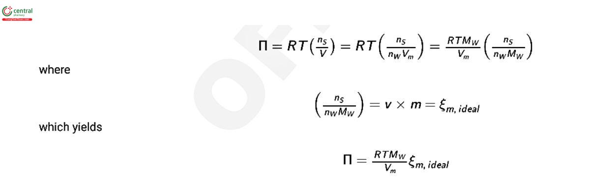
where ns is the moles of solute molecules; nw is the moles of water molecules; V is the volume of water at temperature, T; M is the molar mass of water, M = 18.015268 g mol−1 (3); ξm,ideal is the osmolality of the solution in moles per kilogram of water; ν is the stoichiometric coecient for the solute; and m is the molal concentration of the solute in moles of solute per kilogram of water. For an ideal, nondissociating solute, ν = 1 and the osmolality, ξm , is equal to the molal concentration of solute. For a dissociating solute, ν is equal to the stoichiometric number of moles into which one mole of solute will dissociate. For non-ideal solutes, an osmolality coecient, Φm , is introduced to correct for the difference between the predicted behavior of ideal solutions and the observed behavior of real solutions. The osmolality coecient is dened as:

The osmolality of a real solution is, therefore:
ξm,real = vmΦm
When multiple solutes are present, the osmolality may be approximated by summing the contributions from all individual solutes, i, as:
ξm,real = Σi vimiΦm,i
where m is the molal concentration of the ith solute; ν is the number of ions into which the solute dissociates; and Φm,i is the osmolality coecient for the ith solute at the molality, m. This simplied additive approach assumes that the osmolality coecient for each solute in the mixture is not different from the osmolality coecient determined for the individual solute (4).
In addition to osmotic pressure, other colligative properties can be used to measure the osmolality of solutions including dew-point depression, boiling-point elevation, and freezing-point depression. The most commonly used method for analysis of the osmolality of solutions is freezing-point depression. The freezing-point depression, ΔTf , of an aqueous solution relative to pure water is proportional to the change in the water activity, aw :
ΔTf = (RT2f / ΔHfus) Δln aw
where ΔHfus is the enthalpy of fusion of water, and Tf is the freezing point of the solution in Kelvin. At low solute concentrations, this can be simplied to express freezing-point depression in terms of osmolality as:
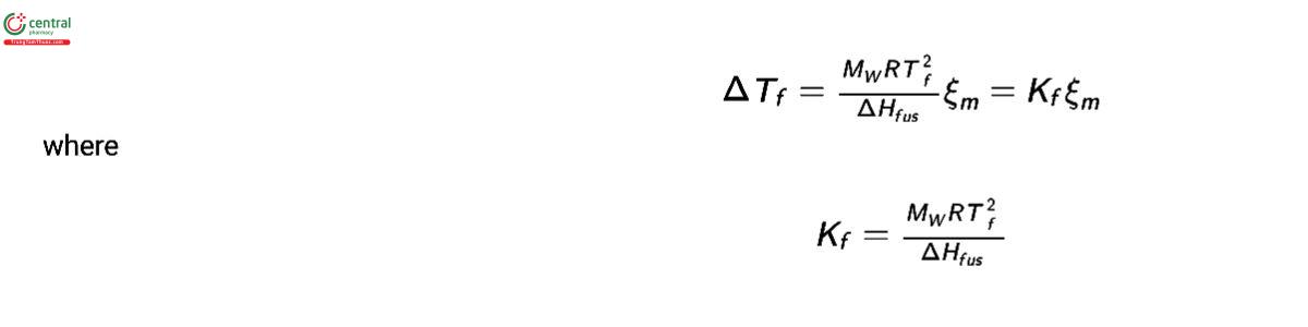
The value of ΔHfus is temperature dependent (3) and so is Kf ; however, Kf is typically treated as a constant and set to the value for pure water at the freezing point. For water, the value of ΔH at 273.15 K is 6006.78 J mol−1 (3), which gives a value for K of 1.86056 K kg mol−1.
Vapor pressure osmometers measure the relative humidity of the air above the sample that is in equilibrium with the sample. The dew point is the temperature below which the water vapor in the air is above saturation and condensation occurs. The change in the dew point of
the air, ΔTD , is given by the Clausius–Clapeyron equation:

where psw is the saturation vapor pressure of the solution; p0sw is the vapor pressure of pure water; and ΔHvap is the enthalpy of vaporization of water. The change in dew point can be expressed in terms of osmolality as:
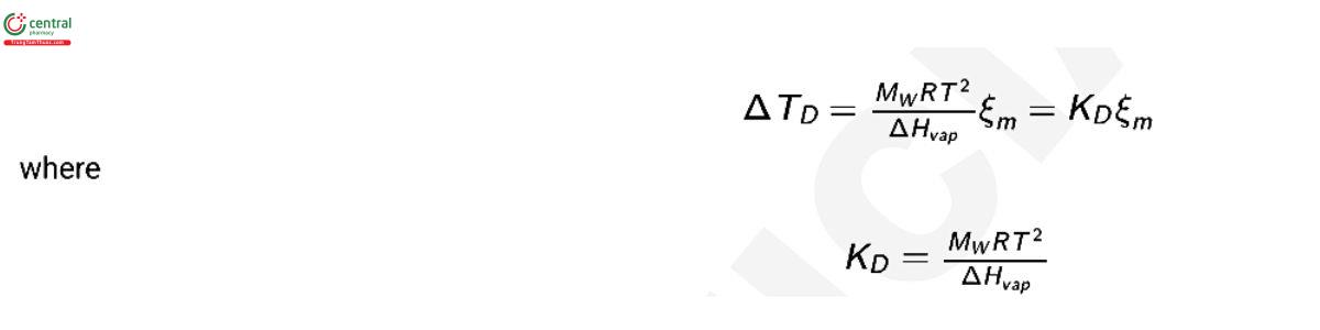
The value of ΔHvap is temperature dependent (5) and so is KD . At 25° (298.15 K), the enthalpy of vaporization of water is ΔHvap = 43.990 k J mol−1 (5) and this results in a value of KD = 0.3027 K kg mol−1. At the boiling point, 373.15 K, ΔHvap = 40.657 k J mol−1 (5) and KD = 0.5130 K kg mol−1 and is equivalent to the ebullioscopic constant, Kb , for water which correlates the osmolality to boiling-point elevation.
To calibrate instruments for measurements of water activity and osmolality, it is necessary to have well-characterized solutions that are easy to prepare. The nonlinear relationship between the osmolality coecient, Φm , and the molality of the solute has been studied for many solutions of single salts and is most often represented by the Pitzer–Debye–Hückel equation (1,4,6) as a virial expansion in terms of molality as follows:
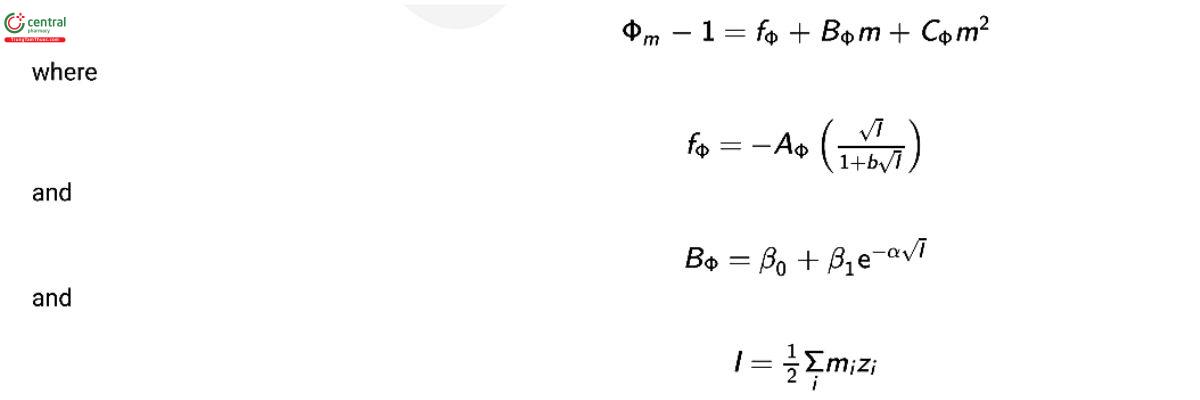
where AΦ is the Debye–Hückel slope; I is the ionic strength; zi is the charge of i; b is the empirical ion size parameter and equal to 1.2; and α is the empirical ionic strength dependence parameter and equal to 2.0. The parameters β0 , β1 , and CΦ are constants that are specic to the particular solute.
For a simple 1:1 electrolyte, like sodium chloride (NaCl), the ionic strength, I, is equal to the molality, and the relationship between molality and osmolality coecient simplies to:
Φm = 1 − AΦ [√m / (1+b√m)] + (β0+ β1e−α√m)
For sodium chloride (NaCl), the value of AΦ has been calculated as a function of temperature and pressure (7), and at 273.15 K and standard pressure, AΦ = 0.37642. Using this value for AΦ and keeping α = 2 and b = 1.2, the remaining values for sodium chloride (NaCl) (β0 , β1 , and CΦ ) can be t to the experimental results for the freezing-point depression of sodium chloride (NaCl) solutions from Scatchard and Prentiss (8) and Gibbard and Gossmann (9). The entire set of experimental results span the range from 2–7300 mOsmol/kg. The resulting best-t parameters of β0 = 0.040933, β1 = 0.26955, CΦ = 0.004506 enable the calculation of recipes for sodium chloride calibration standard solutions for osmolalities within this experimental range. The resulting recipes for Standard Solutions are listed in Table 1. (USP 1-Dec-2020)
Change to read:
3 TYPES OF OSMOLALITY INSTRUMENTS
The osmolality of a solution is commonly determined by measurement of the freezing-point depression or dew-point depression. A freezing-point depression instrument measures the osmolality of a solution at the freezing-point of the solution, whereas a dew-point depression instrument measures the osmolality of a solution at ambient temperatures. Significant changes in the solubility, solvation, and ionization of solutes may occur as temperature changes resulting in a temperature dependence of activity and osmotic coefficients. These factors may lead to significant differences in the osmolality results obtained by different types of osmometers on the same test solutions. Volatile solutes will evaporate during a measurement with vapor pressure osmometers and result in erroneous values. Other techniques need to be used when measuring osmolality in solutions containing volatile solutes.
3.1 Freezing-point Depression Osmometer
A freezing-point depression osmometer typically consists of the following: a means of cooling the container used for the measurement, a thermocouple for measuring the temperature of the sample, and a means of initiating crystallization. The liquid sample (generally about 0.02-2 mL) is typically placed into a cooling bath or a cooling pit while being mixed to facilitate uniform cooling. In small volume freezing-point osmometers (with sample sizes smaller than 100 µL), mixing the liquid is not required for uniform cooling. The sample is supercooled to below the expected freezing point and then a short "buzz" (a brief pulse or shock to initiate crystallization of the water) is applied to the sample. As the sample freezes, the temperature of the thermocouple rises asymptotically toward the freezing point until the sample is completely frozen and the temperature stabilizes. The freezing-point depression is the difference between the freezing point of pure water and the freezing point of the sample.
3.2 Vapor Pressure Osmometer
Vapor pressure osmometers use hygrometric (dew-point temperature depression) measurements for determining water activity. They require a smaller volume of specimen (generally about 5-20 µL). The hygrometric technique is based on measuring the temperature of a wet thermocouple junction in a sealed chamber containing the sample. A current is applied to cool the thermocouple, by means of the Peltier effect, below the dew-point temperature, resulting in condensation of water from the air onto that junction. As water condenses on the thermocouple, the temperature of the thermocouple rises asymptotically toward the dew point. When the temperature of the thermocouple reaches the dew point, condensation ceases, causing the thermocouple temperature to stabilize. The dew-point temperature depression is the difference between the dew-point temperature for air in equilibrium with pure water and the dew-point temperature for air in equilibrium with the sample. In some instruments, the solution to be tested is pipetted onto a small, solute-free paper disk, which is then inserted into the sample chamber containing the thermocouple hygrometer. In other instruments, the solution is tested as a drop at the end of a micropipette inserted into the chamber containing the thermocouple hygrometer. (USP 1-Dec-2020)
Change to read:
4 QUALIFICATION OF OSMOLALITY INSTRUMENTS
Osmometers are classified as Group B instruments as described in Analytical Instrument Qualification (1058). The qualification of an osmometer instrument should cover the intended operational range of the instrument, the required accuracy of the instrument, and the required precision of the instrument. For more details, see (1058). Acceptance criteria for fitness for purpose are based on the uncertainty of the reference material and the performance specification of the instrument. Any osmometer that is shown to be fit for the intended purpose, by meeting the qualification criteria, may be used to provide osmolality results according to the guidelines of this chapter.
4.1 Installation Qualification (IQ)
The installation qualification (IQ) requirements provide evidence that the hardware and software are properly installed in the desired location.
4.2 Operational Qualification (OQ)
The operational qualification (OQ) for the osmolality instrument should characterize the precision and accuracy of the osmolality measurements. Prior to characterizing the performance of the osmolality instrument, perform a full calibration of the instrument, as instructed by the instrument operation manual, and confirm the proper calibration with a calibration check (see Procedure for Calibration Check).
OPTIMIZATION OF ADJUSTABLE FREEZING PARAMETERS
Freezing-point depression osmometers may have user-adjustable parameters that affect the freezing of the Test Solutions. These parameters may include stirring amplitude (during cooling step), "buzz" point (amount of supercooling that precedes initiation of freezing), and "buzz" amplitude (amplitude used to initiate freezing). These test parameters may be optimized, following the manufacturer's recommendations, to reliably freeze the Test Solutions.
PRECISION/REPEATABILITY
The precision of the measurement system should be characterized as part of the operational qualification by performing repeated measurements on the mid-range osmolality standard solution that was used in the instrument calibration. Calculate the sample standard deviation using (n-1) degrees of freedom, o, of six or more measurements, and express the repeatability as a percentage (%) relative to the mean value of the osmolality standard, X0:
R% = 100σ / X0
The precision of the instrument, in mOsmol/kg, at the osmolality of a test solution being analyzed is:
Rosm = (R%/100) X
where X is the mean value for the test solution. After characterizing the precision of the measurement system, this result should be compared to the manufacturer's claimed repeatability. If the result is significantly greater than the claimed repeatability (e.g., more than twice the claimed repeatability), then the performance of the osmometer should be more fully investigated. The acceptance criterion is that the relative standard deviation should be NMT 2%.
ACCURACY
Verify the accuracy of the calibrated instrument by measurement of at least three replicates of the highest and lowest osmolality standard used during the calibration. The instrument reading should be within ±4 mOsmol/kg of the stated value for the standard solutions up to 400 mOsmol/kg and within ±1% of the stated value for the standard solutions >400 mOsmol/kg.
4.3 Performance Qualification (PQ)
The performance qualification (PQ) should be evaluated by periodic recalibration of the instrument and a day-of-use calibration check. It is recommended that the result for the day-of-use calibration check be monitored over time to track performance of the instrument. (USP 1-Dec 2020)
Change to read:
5 OPERATION AND CALIBRATION OF OSMOMETERS
5.1 Standard Solutions
Solutions for instrument calibration may be purchased (10) or may be prepared as specified in Table 1. Other concentrations not listed in Table 1 are acceptable. They may be stored at 2°–30°, but should not be frozen. When using purchased solutions, follow the manufacturer's expiry date and use instructions. Purchased solutions are typically provided in single-use ampules and should be discarded after use. Solutions prepared as specified in Table 1 should be stored in nonpermeable (e.g., glass) containers to prevent evaporation. Fresh solutions should be prepared at least monthly as they are often nonsterile unpreserved solutions.
Table 1. Standard Solutions (STD) for Freezing-Point Depression Osmometer Calibrationa,b
| mOsmol/kg of STD | g of Sodium Chloride/kg of Water | mOsmol/kg of STD | g of Sodium Chloride/kg of Water |
| 50 | 1.530 | 1600 | 51.39 |
| 100 | 3.098 | 1700 | 54.58 |
| 150 | 4.683 | 1800 | 57.76 |
| 200 | 6.278 | 1900 | 60.92 |
| 250 | 7.880 | 2000 | 64.08 |
| 290 | 9.165 | - | - |
| 300 | 9.487 | 2100 | 67.23 |
| 350 | 11.10 | 2200 | 70.36 |
| 400 | 12.71 | 2300 | 73.48 |
| 450 | 14.33 | 2400 | 76.59 |
| 500 | 15.94 | 2500 | 79.69 |
| 550 | 17.56 | 2600 | 82.78 |
| 600 | 19.18 | 2700 | 85.85 |
| 650 | 20.80 | 2800 | 88.91 |
| 700 | 22.41 | 2900 | 91.95 |
| 750 | 24.03 | 3000 | 94.98 |
| 800 | 25.65 | 3100 | 98.00 |
| 850 | 27.27 | 3200 | 101.00 |
| 900 | 28.89 | 3300 | 103.99 |
| 950 | 30.50 | 3400 | 106.96 |
| 1000 | 32.12 | 3500 | 109.92 |
| 1100 | 35.35 | 3600 | 112.86 |
| 1200 | 38.57 | 3700 | 115.79 |
| 1300 | 41.79 | 3800 | 118.70 |
| 1400 | 45.00 | 3900 | 121.60 |
| 1500 | 48.20 | 4000 | 124.48 |
a Calculated from experimental data from Scatchard and Prentiss (8) and Gibbard and Gossmann (9) with best-t parameters of AΦ = 0.37642; β0 = 0.040933; β1 = 0.26955; CΦ = 0.004506; α = 2, b = 1.2.
b The amount of sodium chloride (NaCl) specied is added to 1 kg of water (on weight basis). Weigh sodium chloride (NaCl), which has been previously dried at 110° for 2 h, to ±0.03 g and weigh water to ±0.2 g to ensure osmolality is accurate to correct whole number of mOsmol/kg. If correctly prepared, the accuracy of these Standard Solutions is ±1 mOsmol/kg. For purchased solutions, the accuracy is typically ±2 mOsmol/kg for concentrations up to 400 mOsmol/kg, and ±0.5% for concentrations >400 mOsmol/kg. Other Standard Solution concentrations can be prepared as needed.
5.2 Calibration
The osmometer should be calibrated as per the manufacturer's instructions using either purchased or prepared Standard Solutions (as described in Table 1).
PROCEDURE FOR CALIBRATION CHECK
The calibration check should be performed in the same manner that measurements will be performed. If individual measurements will be reported, the calibration check should be performed with a single measurement of a standard solution. If the mean of three measurements will be reported, the calibration check should be performed with the mean of three measurements of a standard solution. Unless a different solution is specified as part of the manufacturer's instructions, select at least one solution from Table 1 that lies near the center of the expected range of osmolality for the test solution. Two Standard Solutions bracketing the test sample within 300 mOsmol/kg are also acceptable. The instrument reading should be within ±4 mOsmol/kg from the stated value for solutions ≤400 mOsmol/kg and within ±1% from the stated value for solutions >400 mOsmol/kg. If the instrument fails to meet the acceptance criteria for the calibration check, then calibrate the instrument as per the manufacturer's instructions using either purchased or prepared Standard Solutions (as described in Table 1), and then repeat the calibration check of the instrument. After a successful check of the calibration, the instrument is ready for use.
5.3 Test Solutions
For a solid for injection, reconstitute with the appropriate diluent as specified in the instructions on the labeling. For solutions, use the sample as is. [NOTE-A solution can be diluted to bring it within the range of measurement of the osmometer, if necessary, but the results must be expressed as those of the diluted solution and must NOT be multiplied by a dilution factor to calculate the osmolality of the original solution unless otherwise indicated in the monograph. The molal osmotic coefficient is a function of concentration and changes nonlinearly with dilution.] Unless otherwise directed in the monograph, use Method 1.
5.4 Method 1: Freezing-Point Osmometry
PROCEDURE
Verify that the instrument has been turned on for an appropriate amount of time (NLT 30 min unless the instrument contains an internal sensor) to enable the cooling bath to equilibrate to its normal operating temperature. Verify that the calibration of the instrument brackets the expected osmolality of the test solution. If not, perform a new calibration of the instrument such that the lower and upper calibration standards bracket the expected osmolality of the samples to be evaluated. At least each day of use, confirm the instrument calibration as described in Procedure for Calibration Check. Before each measurement, rinse the measurement cell with the solution to be tested, and verify that the thermocouple is clean and dry before immersing it into the test solution.
TROUBLESHOOTING
Samples may sometimes fail to freeze if the sample viscosity is too high, if the sample is precooled too much or not enough, or if the mixing speed or the amplitude of the instrument is not optimally set. If test solutions occasionally fail to freeze, the osmolality measurements may not be accurate. The settings of the instrument should be optimized to reliably freeze the test solution, and then the instrument should be recalibrated with the optimized settings prior to re-evaluation of the test solutions.
Insoluble particles, emulsified droplets that are insoluble and entrained air, will not significantly affect the osmolality of the aqueous vehicle; however, these may affect the ability of the sample to freeze. If accurate measurement of the osmolality is affected by the presence of the insoluble phase, the insoluble phase should be removed by centrifugation and the osmolality of the clarified aqueous phase should be evaluated and reported.
5.5 Method 2: Vapor Pressure Osmometry
STANDARD SOLUTIONS
The osmolality reference standards in Table 1 are based on freezing-point depression measurements (8,9) and represent the osmolality of the solution at the freezing point. However, manufacturers of dew point osmometers often typically design their instruments to be calibrated with the same standard solutions used for freezing-point depression instruments. Unless otherwise directed by the instrument manufacturer, it is permitted to use the same Standard Solutions that were defined above for use with the freezing-point depression instruments. When performing an instrument calibration and calibration check with these Standard Solutions, the stated value for the standard solution is considered to be the same as indicated for the freezing-point depression instruments.
PROCEDURE
Ensure that the sample and instrument are located in a laboratory with good temperature control and that the sample is equilibrated to the temperature of the laboratory before performing the measurement. Verify that the instrument has been turned on for NLT 30 min to completely equilibrate to the lab temperature while operating. Verify that the calibration of the instrument brackets the expected osmolality of the test solution. If not, perform a new calibration of the instrument such that the lower and upper calibration standards bracket the expected osmolality of the samples to be evaluated. At least each day of use, confirm the instrument calibration as described in Procedure for Calibration Check. If the sample is dispensed for the measurement by a pipette, use a calibrated pipette to deliver the specified volume of liquid to the sample chamber. Consistent timing during sample loading is important for consistent repeatability. The procedure and timing for sample loading need to be equivalent to those used for the instrument calibration.
TROUBLESHOOTING
Volatile ingredients (e.g., Ethanol) may evaporate rapidly during the sample loading and measurement resulting in inaccurate and variable results. (USP 1-Dec-2020)
Change to read:
6 REPORTING OF RESULTS
6.1 Units
The units of osmolality are osmole per kilogram of water (Osmol/ kg ) or milliosmole per kilogram of water (mosmol/ kg ) . The units of osmolarity are osmole per liter of solution (Osmol/ L ) or milliosmole per liter of solution (mosmol/ L ) It is not necessary to state "of water" or "of solution" when using these units. The use of "Osmol" alone must be avoided because it is not clear whether it refers to the number (osmoles of solute) or the osmolality or the osmolarity.
6.2 Measurement Result
If a single measurement result is reported, it should be reported with the precision given by the repeatability of the instrument. Preferably, the mean of three or more measurements on the same solution should be reported with a precision represented by the standard deviation of the averaged measurements. Most osmometers report results to the nearest whole number, therefore, the mean result should also be rounded to the nearest whole number and reported in units of mosmol/kg.
6.3 Conversion to Osmolarity
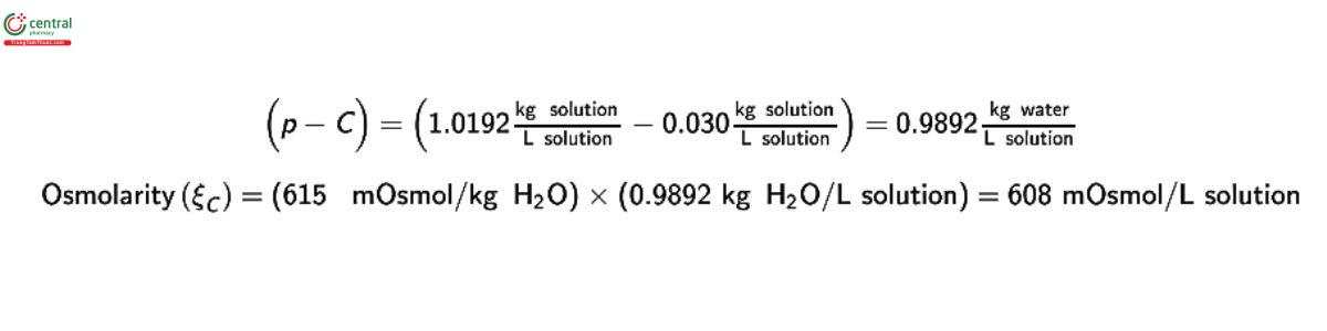
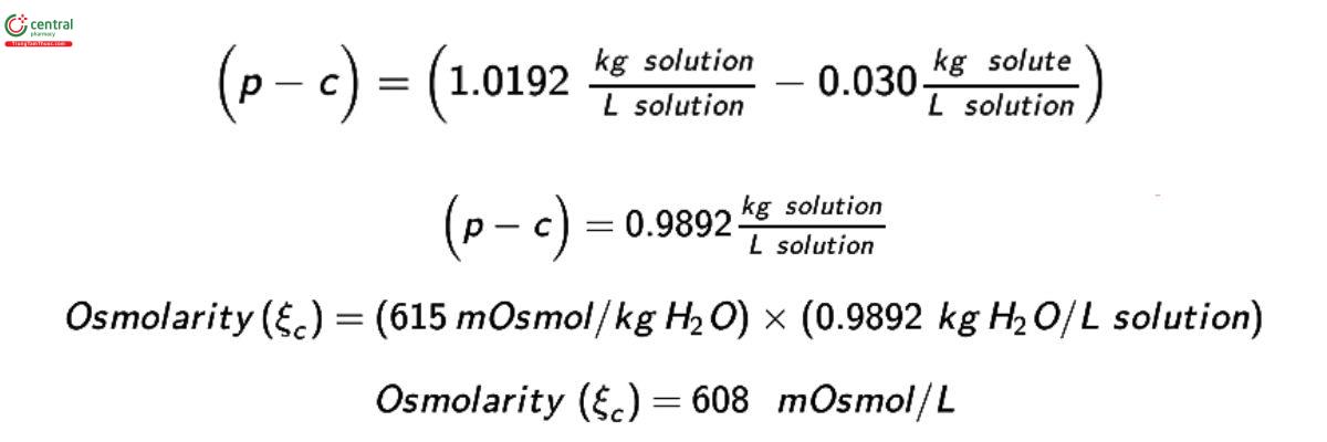
Freezing-point depression and vapor pressure measurements directly result in an assessment of the osmolality. However, it may be desirable to report the results in units of osmolarity. The measured osmolality ( ξm) can be converted to osmolarity (ξc) using:
ξc = ξm (p - C)
where p is the density of the solution and C is the total solute concentration, both expressed in grams per milliliter.
Example of conversion to osmolarity:
A 3% (w/v) solution of sodium bicarbonate contains 0.030 g/mL of anhydrous sodium bicarbonate. The density of this solution was found to be 1.0192 g/mL at 20°, and its measured osmolality (m) was 615 mosmol/kg.
[NOTE-1 g/mL = 1 kg/L.]
6.4 Tonicity
Tonicity is a medical term that relates to the osmotic pressure difference between the internal and external sides of a cell membrane. In many cases tonicity and osmolality are not the same because some solutes are able to rapidly pass through the cell membrane. Red blood cells, erythrocytes, are typically considered the standard for defining what is considered an isotonic solution. If red blood cells are immersed in a solution and the cells swell and become turgid or burst, the solution is hypotonic. If the red blood cells shrink and desiccate, the solution is hypertonic. An isotonic solution produces no change in the size of the red blood cells and the cell wall remains flaccid. Measurements of osmolality or osmolarity alone are not sufficient to characterize the tonicity of a liquid. It is preferable to use the terms hypoosmotic, hyperosmotic, and isoosmotic when discussing the relative osmolality of solutions. The standard for an isoosmotic solution is 0.9% sodium chloride (NaCl) solution, which has an osmolality of 285 mOsmol/kg and an osmolarity of 284 mOsmol/L. (USP 1-Dec-2020)
Delete the following:
7 OSMOLARITY
Osmolarity of a solution is a theoretical quantity expressed in osmoles/L (Osmol/L) of a solution and is widely used in clinical practice because it expresses osmoles as a function of volume. Osmolarity cannot be measured but is calculated theoretically from the experimentally measured value of osmolality.
Sometimes, osmolarity (ξc ) is calculated theoretically from the molar concentrations:
ξc = Σνi ci
νi = number of particles formed by the dissociation of one molecule of the ith solute
ci = molar concentration of the ith solute in solution
For example, the osmolarity of a solution prepared by dissolving 1 g of Vancomycin in 100 mL of 0.9% sodium chloride solution can be calculated as follows:
[3 x 10 g/L/1449.25(molecular weight of vancomycin) + 2 x 9 g/L/58.44(molecular weight of sodium chloride)] x 1000 = 329 mOsmol/L
The results suggest that the solution is slightly hyperosmotic because the osmolality of blood ranges between 285 and 310 mOsmol/kg. However, the solution is found to be hypoosmotic and has an experimentally determined osmolality of 255 mOsmol/kg.1 The example illustrates that osmolarity values calculated theoretically from the concentration of a solution should be interpreted cautiously and may not represent the osmotic properties of infusion solutions.
The discrepancy between theoretical (osmolarity) and experimental (osmolality) results is, in part, due to the fact that the osmotic pressure of a real solution is less than that of an ideal solution because of interactions between solute molecules or between solute and solvent molecules in a solution. Such interactions reduce the pressure exerted by solute molecules on a semipermeable membrane, reducing experimental values of osmolality compared to theoretical values. This difference is related to the molal osmotic coefficient (m). The example also illustrates the importance of determining the osmolality of a solution experimentally, rather than calculating the value theoretically.
To convert to osmolality, it is necessary to know the kilogram of water per liter of solution as the conversion factor. The density of the solution should be measured and the amount of (anhydrous) solute per unit of volume should be known based on the preparation of the solution. If working with an unknown solution, the value of a loss on drying measurement could also be used (assuming water is the only volatile component in the solution).
Example 1: A 3% (w/v) solution of sodium bicarbonate contains 0.030 g/mL of anhydrous sodium bicarbonate. The density of this solution was found to be 1.0192 g/mL at 20°, and its measured osmolality was 615 mOsmol/kg. [NOTE-1 g/mL = 1 kg/L.]
Example 2: An aqueous solution sodium lauryl sulfate (SLS) as raw material has a content of 30% (on a w/v basis) and has a specic gravity of 1.08 g/mL at 20°. It also contains 0.5% of sodium sulfate (Na2SO4). Calculate the predicted osmolarity and convert this into expected osmolality, if it is evaluated (assume an ideal solute, Φm = 1.0). The molecular weight of SLS is 288.37 g/mol. The molecular weight of sodium sulfate (Na2SO4) is 142.04 g/mol. The density of the material at 20° is 1.08/0.997 = 1.083 g/mL.
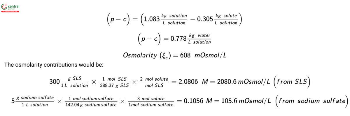
Total osmolarity = 2080.6 + 105.6 = 2186.2 mOsmol/L (USP 1-Dec-2020)
Delete the following:
8 MEASUREMENT OF OSMOLALITY
The osmolality of a solution is commonly determined by the measurement of the freezing point depression of the solution.
8.1 Apparatus
The apparatus, an osmometer for freezing point depression measurement, consists of the following: a means of cooling the container used for the measurement; a temperature measuring device with an appropriate current- or potential-difference measurement device that may be graduated in temperature change or in osmolality; and a means of mixing the sample.
Osmometers that measure the vapor pressures of solutions are less frequently employed. They require a smaller volume of specimen (generally about 5 µL), but the accuracy and precision of the resulting osmolality determination are comparable to those obtained by the use of osmometers that depend upon the observed freezing points of solutions.
8.2 Standard Solutions
Prepare Standard Solutions as specified in Table 1, as necessary.2
Once prepared, the Standard Solutions may be stored in nonpermeable container-closure systems. They should be prepared fresh every week as they are nonsterile, unpreserved solutions. If using purchased solutions, follow the manufacturer's expiration date.
Table 1. Standard Solutions for Osmometer Calibrationa
| Standard Solutions (Weight in g of sodium chloride per kg of water) | Osmolality (mOsmol/kg) (ξm) | Molal Osmotic Coecient (Φm, NaCl) | Freezing Point Depression (°) ΔTf |
| 3.087 | 100 | 0.9463 | 0.186 |
| 6.260 | 200 | 0.9337 | 0.372 |
| 9.463 | 300 | 0.9264 | 0.558 |
| 12.684 | 400 | 0.9215 | 0.744 |
| 15.916 | 500 | 0.9180 | 0.930 |
| 19.147 | 600 | 0.9157 | 1.116 |
| 22.380 | 700 | 0.9140 | 1.302 |
a Adapted from the European Pharmacopoeia, 4th Edition, 2002, p. 50
8.3 Test Solution
For a solid for injection, constitute with the appropriate diluent as specied in the instructions on the labeling. For solutions, use the sample as is.
[Note—A solution can be diluted to bring it within the range of measurement of the osmometer, if necessary, but the results must be expressed as that of the diluted solution and must NOT be multiplied by a dilution factor to calculate the osmolality of the original solution, unless otherwise indicated in the monograph. The molal osmotic coecient is a function of concentration. Therefore, it changes with dilution.]
8.4 Procedure
First, calibrate the instrument by the manufacturer's instructions. Conrm the instrument calibration with at least one solution from Table 1 such that the osmolality of the Standard Solution lies within 50 mOsmol/kg of the expected value of the Test Solution or the center of the expected range of osmolality of the Test Solution. The instrument reading should be within ±4 mOsmol per kg from the Standard Solution. Introduce an appropriate volume of each Standard Solution into the measurement cell as in the manufacturer's instructions, and start the cooling system. Usually, the mixing device is programmed to operate at a temperature below the lowest temperature expected from the freezing point depression. The apparatus indicates when the equilibrium is attained. If necessary, calibrate the osmometer, using an appropriate adjustment device such that the reading corresponds to either the osmolality or freezing point depression value of the Standard
Solution shown in Table 1.
[Note—If the instrument reading indicates the freezing point depression, the osmolality can be derived by using the appropriate formula under Osmolality.]
Repeat the procedure with each Test Solution. Read the osmolality of the Test Solution directly, or calculate it from the measured freezing point depression.
Assuming that the value of the osmotic coecient is essentially the same whether the concentration is expressed in molality or molarity, the experimentally determined osmolality of a solution can be converted to osmolarity in the same manner in which the concentration of a solution is converted from molality to molarity. Unless a solution is very concentrated, the osmolarity of a solution (ξc ) can be calculated as follows:
ξc = 1000ξm /(1000/ρ + Σwi νi )
ξm = experimentally determined osmolality
ρ = density of the solution
wi = weight (g)
νi = partial specic volume of the ith solute (mL/g)
The partial specic volume of a solute is the change in volume of a solution when an additional 1 g of solute is dissolved in the solution. This volume can be determined by the measurement of densities of the solution before and after the addition of the solute. The partial specic volumes of salts are generally very small, around 0.1 mL/g. However, those of other solutes are generally higher. For example, the partial specic volumes of amino acids are in the range of 0.6–0.9 mL/g. It can be shown from the above equation correlating osmolarity with osmolality that:
ξc = ξm (ρ−c)
ξm = experimentally determined osmolality
ρ = density of the solution (g/mL)
c = total solute concentration (g/mL)
Thus, alternatively, the osmolarity can also be calculated from experimentally determined osmolality from the measurement of density of the solution by a suitable method and the total weight of the solute, after correction for water content, dissolved per milliliter of the solution. (USP 1-Dec-2020)
Change to read:
9 REFERENCES
1. Pitzer KS, Pelper JC, Busey RH. Thermodynamic properties of aqueous sodium chloride solutions. J Phys Chem Ref Data. 1984;13(1).
2. Mohr PJ, Newell DB, Taylor BN. CODATA recommended values of the fundamental physical constants: 2014. Rev Mod Phys. 2016;88.
3. Feistel R, Wagner W. A new equation of state for H O Ice Ih. J Phys Chem Ref Data. 2006;35(2).
4. Prickett RC, Elliott JAW, McGann LE. Application of the multisolute osmotic virial equation to solutions containing electrolytes. J Phys Chem B. 2011;115:14531–14543.
5. Marsh KN, ed. Recommended reference materials for the realization of physicochemical properties. Pure Appl Chem. 1980;52:2393– 2404.
6. Partanen JI. Mean activity coecients and osmotic coecients in dilute aqueous sodium or potassium chloride solutions at temperatures from (0 to 70)°C. J Chem Eng Data. 2016;61(1):286–306.
7. Archer DG, Wang P. The dielectric constant of water and Debye-Hückel limiting law slopes. J Phys Chem Ref Data. 1990;19:371.
8. Scatchard G, Prentiss SS. The freezing points of aqueous solutions. IV. Potassium, sodium and lithium chlorides and bromides. J Am Chem Soc. 1933;55:4355.
9. Gibbard HF, Gossmann AF. Freezing points of electrolyte mixtures. I. Mixtures of sodium chloride and magnesium chloride in water. J Solution Chem. 1974;3(5):385–393.
10. Commercially available solutions for osmometer calibration, with osmolalities equal to or different from those listed in Table 1 and standardized by methods traceable to the National Institute of Standards and Technology (NIST) (www.nist.gov) or any other national or international standards setting organizations may be used. [Note—A possible supplier for those solutions is Advanced Instruments Calibration Standards available from www.aicompanies.com or www.vwr.com.] (USP 1-Dec-2020)
1 Kastango ES, Hadaway L. New perspectives on vancomycin use in home care, part 1. Int J Pharm Compd. 2001;5(6):465–469.
2 Commercially available solutions for osmometer calibration, with osmolalities equal to or different from those listed in Table 1 and standardized by methods traceable to National Institute of Standards and Technology (NIST) (www.nist.gov), may be used.
