Measurement of Yield Stress of Semisolids

This article is compiled based on the United States Pharmacopeia (USP) – 2025 Edition

Issued and maintained by the United States Pharmacopeial Convention (USP)

DOWNLOAD PDF HERE

1 BACKGROUND

Semisolids are viscoelastic materials that exhibit a yield stress. The yield stress for a raw material or dosage form1 is the applied stress at which a change in the viscoelastic properties of a semisolid is observed: below the yield stress the material response is dominated by completely reversible elastic deformation, whereas above the yield stress the material response is changing to irreversible elastic behavior (as the material remains a viscoelastic semisolid) or is dominated by viscous flow behavior. Often, the yield stress is identified as the applied stress below which a material appears to not show any motion or flow (i.e., where the shear rate is near-zero).

This observation can be dependent on the sample preparation, methods of testing and analysis, the time scale of the measurement, the scan rate used to locate the change in the behavior, and the direction from which the transition is approached. Most rotational measurement techniques identify the yield stress by locating the onset of flow; however, penetrometry, which is another rheological technique, looks for the yield stress where the semisolid stops yielding. Although the yield stress for various materials is expected to correlate when measured with different techniques, the values should not be considered to be independent of the method of testing and analysis. Yield stress is reported with units of shear stress [Pascals (Pa)].

Characterizing and monitoring the viscoelastic properties of semisolids is not straightforward because the properties can be dominated by either solid- or liquid-like behavior depending on how much deformation or stress is applied to the material. If the quality of a raw material or dosage form is primarily dependent on the behavior under high-shear conditions, then viscosity may be an appropriate parameter to monitor. In this case, efforts should be made to avoid wall slip and make measurements where the applied shear stress is much greater than the yield stress. However, if the properties of the raw material or dosage form are critical to quality at low shear or at rest (e.g., uniformity and stability of an ointment suspension or residence time at site of application), then measurement of the yield stress using one or more of the methods described below may be required.

For temperature-sensitive materials, viscoelastic properties at both ambient conditions (i.e., storage conditions) and physiological conditions [i.e., skin surface temperature (32°) or body temperature (37°)] are useful. For example, an anesthetic topical cream may require characterization at 32°, whereas a vaginal cream may require characterization at 37° (1–2).

A brief summary of the mathematical models used to quantify the viscoelastic properties of semisolids is presented below, followed by a summary of the most common experimental methods for assessing the viscoelastic properties and determining the yield stress for semisolids. [NOTE—Additional models for viscosity versus shear rate are also discussed in Rheometry 〈1911〉, see Figure 3).]

1.1 Hooke’s Elasticity Law and Newton’s Viscosity Law

For elastic materials, Hooke’s Elasticity Law applies,

σ = Gγ    Equation 1

where σ is the shear stress (= force/surface area, in units of pascals, Pa), G is the shear modulus that represents the rigidity of a material, and γ is the shear strain or shear deformation (= displacement/distance or shear gap, dimensionless).

For viscous materials, Newton’s Viscosity Law applies,

σ = ηγ⋅     Equation 2

where σ is the shear stress, η is the shear viscosity that represents the resistance of the material to flow, and γ⋅ is the shear rate (or strain rate = velocity/distance or shear gap, in units of s⁻¹).

Semisolid raw materials and dosage forms will have both viscous and elastic properties and, hence, are categorized as viscoelastic materials.

1.2 Herschel–Bulkley Equation

The Herschel–Bulkley equation is suitable for parameterizing the observed shear stress versus shear rate information for a wide range of viscoelastic materials including semisolids exhibiting a yield stress. The Herschel–Bulkley equation is:

σ = κγ^η + σ_γ      Equation 3

where, σ is the shear stress, κ is the proportionality constant (formerly also referred to as consistency), γ⋅ is the shear rate, η is the exponent, and σ_γ is the yield stress according to Herschel–Bulkley.

The exponent, n, is less than 1 for shear-thinning fluids and is greater than 1 for shear-thickening fluids.

When n = 1, the Herschel–Bulkley equation simplifies to the Bingham equation with κ referred to as the Bingham viscosity. When n = 0.5, the Herschel–Bulkley equation simplifies to the Casson equation with κ typically referred to as the Casson viscosity.

1.3 Oscillatory Measurements of Viscoelastic Properties

If a sinusoidal oscillating shear strain (shear deformation) is applied to a material,

γ(t) = γ₀ sin(ωt)      Equation 4

where γ(t) is the amplitude at time (t), γ₀ is the amplitude at time zero, and ω is the angular frequency of the shear strain, the corresponding shear rate is calculated as follows.

γ(t) = γ₀ω cos(ωt) = γ₀ cos(ωt)    Equation 5

According to Hooke’s Elasticity Law, the ideal elastic response to this applied shear strain will be sinusoidal: 

σ(t) = γ₀G sin(ωt)       Equation 6

 which indicates that the ideal elastic response is in-phase with the strain (G is the shear modulus). According to Newton’s Viscosity Law, the ideal viscous response will also be sinusoidal:

 σ(t) = ηγ₀ω cos(ωt)       Equation 7

which indicates that the ideal viscous response is out-of-phase (shifted by 90°, showing the phase shift angle of δ = 90°) relative to the shear strain.

For a viscoelastic material, the response will be sinusoidal with a phase shift angle, δ (also referred to as the loss angle) of 0° ≤ δ ≤ 90°.

σ(t) = σ₀ sin(ωt + δ)        Equation 8

The response of a viscoelastic material to an applied sinusoidal shear strain is used to determine the values of the loss angle, δ, and the amplitude of the response, σ . This response can be separated into a viscous and elastic component according to Equation 9 and Equation 10,

G ′ = (σ₀/γ₀) cos δ          Equation 9

G ′′ = (σ₀/γ₀) sin δ          Equation 10

where G′ is called the elastic (storage) modulus and G″ is called the viscous (loss) modulus. The dimensionless loss factor (or damping factor) as the ratio of the viscous and the elastic portions is defined as: tan δ = G″/G′ (unit: 1).

Therefore, the sinusoidal response of a viscoelastic material to an oscillatory shear strain (or shear stress) can be used to separate the viscous and elastic responses for a semisolid material in the range of low strains and low stresses without requiring the material to actually flow.

When the elastic response of a material is dominant (G′ > G″), the material is referred to as a viscoelastic solid or a gel. When the viscous response of a material is dominant (G′ < G″), the material is referred to as viscoelastic liquid or a sol. The point where G′ = G″ (tan δ = 1) is referred to as the sol–gel transition.

2 EXPERIMENTAL METHODS

2.1 Yield Stress via the Viscosity Maximum

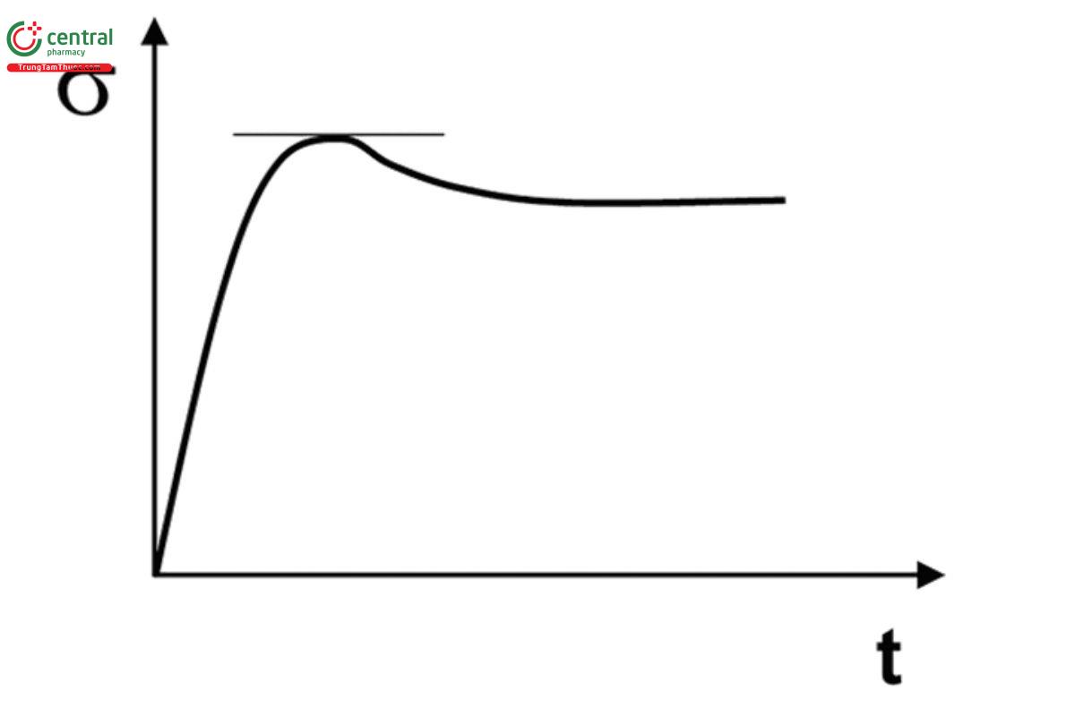
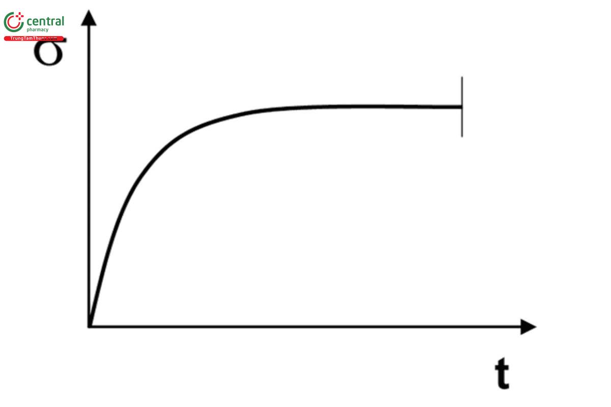
A viscosity maximum is performed by presetting a constant, very low ("near-zero") shear rate (e.g., of 0.01 or 1 s−1) or a very low rotational speed (e.g., of 0.01 or 1 rpm). The relationship between rotational speed n (in rpm) and angular velocity ω (in rad/s or 1/s) is: ω = (2π/60) × n. As a result, the yield stress corresponds to the maximum viscosity (or shear stress or torque), which can be displayed in a diagram showing one of these parameters on the y-axis and time (or shear strain) on the x-axis. The following applies according to Newton's Viscosity Law (see Equation 2): Because this experiment is run at a constant shear rate (or speed), the shear viscosity and the shear stress are proportional. The shape of the plots of the shear viscosity and shear stress (or torque) are identical. The resulting viscosity (or shear stress or torque) values will begin to increase with time (transient viscosity function, i.e., time-dependent). When approaching the yield stress, the increase in the values will slow, and thus, the curve will become flatter. There are two possible results:

The plot will clearly show a maximum (or peak). The yield point (in Pa) is read off as the shear stress value appearing at the maximum point of the curve (see Figure 1A).

The plot will steadily approach to a (constant) plateau value. The yield point (in Pa) is read off as the shear stress value when first reaching the plateau value (see Figure 1B).

The experimental parameters that influence this measurement method include the sample loading technique, the placement of the measurement geometry (often a vaned rotor) in the sample cup, and the sample history. Because air pockets may be of concern, ideally, the sample should be loaded gently, without significant shearing and without introducing any air, and the sample cup should be large enough that the vane or cylinder can be placed at least 2H above the bottom of the sample cup (where H is the height of the vane or cylinder) and at least a distance D away from the side of the sample cup (where D is the diameter of the vane or cylinder). To avoid end effects at the top of the vaned rotor or cylinder, either the top should be at least H/2 below the air interface, or the geometry should be positioned so that the top is at or above the air interface. After carefully immersing the geometry into the sample, an equilibration time may be required to relieve any stresses developed during the loading of the sample. The yield stress may be affected by the shear rate (or speed) used. When comparing different raw materials or dosage forms, it is important and recommended to use the same measurement speed.

2.2 Yield Stress via Shear Rate Ramps or Shear Stress Ramps (flow curves)

The yield stress of a material can be estimated in two ways:

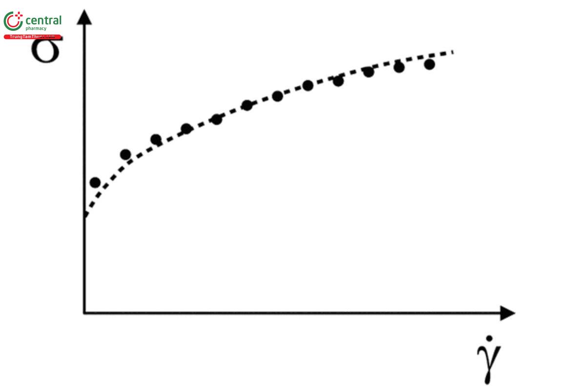
Using a non-linear regression approach based on the Herschel–Bulkley equation (Equation 3), see Figure 2.

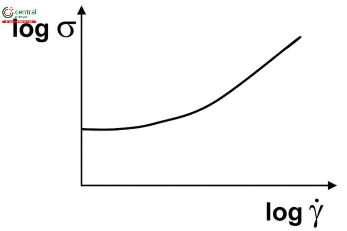
Reading the plateau value at low shear rate. As shown in Figure 3, a material with a yield stress will exhibit a plateau on this log–log plot and the yield stress will correspond to this asymptotic value at low shear rate. If the plateau is not apparent, then fitting to the Herschel–Bulkley equation will provide a better estimate of the yield stress.

Modern rotational rheometers can perform flow curve measurements using two modes of operation: 1) controlled shear rate (CSR) and 2) controlled shear stress (CSS). For CSR, typical examples for testing include: a) on a linear scale, preset of 20 measuring points from shear rate 0 to 1000 s−1; and b) on a logarithmic scale, preset of 10 measuring points per decade between 0.01 s⁻¹ (or 1 s⁻¹) and 1000 s⁻¹.

For these experiments, wall slip at low shear rates will significantly affect the results. It is highly recommended that either a vaned rotor or a roughened (e.g., cross-hatched) parallel plate (PP) measurement geometry be used. In extreme cases of wall slip, a material with a yield stress may appear to switch to a state of flow and may lead to the incorrect conclusion that the material does not exhibit any yield stress at all. One benefit of dynamic oscillation stress or strain sweep tests is that it provides a lower probability of wall slippage.

2.3 Yield Stress by Amplitude Sweep

For oscillatory measurements in the form of amplitude sweeps, the amplitude of the shear strain (or shear stress) is increased from low to high on a logarithmic scale (e.g., shear strain from 0.01%–100% or shear stress from 1 to 1000 Pa, preset on a log scale, with 10 points per decade). Users often perform amplitude sweeps at ω = 10 rad/s (or, alternatively, at frequency (f) = 1 Hz). This test may be used to evaluate the viscoelastic behavior and the stiffness (rigidity) of a gel in the linear viscoelastic range (LVR) . The LVR is the low shear range where the response of a sample behaves predominantly according to Hooke’s Elasticity Law, the shear strain (shear deformation) is reversible, and the resulting parameters (G′ and G″) are constant, both showing plateau values with G′ > G″ within this region. The LVR limit typically is determined in terms of the shear strain or shear stress value when the G′ curve deviates from the plateau value by 5% (see ISO 3219-3 for more information), usually downward.

The yield stress value is correlated with the storage modulus drop that occurs beyond the limit of the LVR. The limit of the LVR may be considered the onset of yielding or, alternatively, the onset point for yielding may be located as the intersection of an initial tangent line (from the LVR) with a final tangent line (where the G' curve or complex viscosity drops rapidly). Additionally, the G′ and G″ crossover point may be considered a transition from elastic to viscous behavior. A yield point or yield stress may be identified from these plots in multiple ways.

Because the oscillatory tests do not require the measuring sample to flow, wall slip may not be a significant concern for these experiments, although vaned rotor and roughened measurement geometries may still be used.

Each amplitude sweep is performed at a single frequency. [For the conversion between the angular frequency ω (in rad/s) and the frequency (in Hz): ω = 2π × f.] The frequency selected for the amplitude sweep will affect the value of G′ in the LVR and may affect the location of the crossover point of the curves of G′ and G″.Frequency sweeps may be performed to determine the significance of the frequency (or time) dependence of the results.

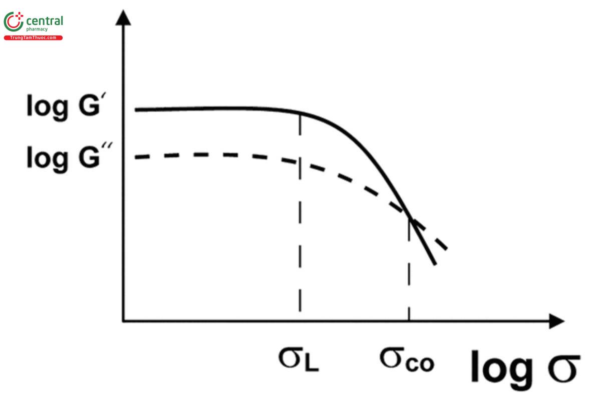
Figure 4 shows an example of an amplitude sweep of a typical semisolid. In the LVR, the G′ value of the material is constant and may be used as a measure of the stiffness of the material. At the limit of the LVR, the value of G′ begins to depart from the plateau, typically by sloping downward, and at even higher strain (or stress) amplitudes, the material exhibits the crossover point of G′ and G″. Both the limit of the LVR and the crossover point of G′ and G″ represent significant changes in the viscoelastic properties of the material that sometimes are selected as a yield stress value. This can be interpreted as follows:

The limiting shear stress, or σ , is the shear stress at the limit of the LVR. At this limit, the semisolid begins to yield but G′ still dominates G″, and thus the elastic (solid) behavior over the viscous (liquid) one.

The shear stress at the crossover point (also known as the flow point), or σ , is the point where G″ dominates G′, and thus, the viscous (liquid) behavior over the elastic (solid) one. In other words, at this point the material is predominantly in a flowing state. Many practical users prefer the crossover point for two reasons: It can be located more precisely as it occurs clearly as a single point in the diagram, and it has been found to correlate particularly with the yield stress values resulting from rotational tests. [NOTE—However, for amplitude sweeps, the values of the crossover point (G′ = G″) in terms of the shear strain and shear stress are clearly measured outside of the LVR.]

2.4 Penetrometry Measurements

In the penetrometry experiment, a cone with an angle of 2α is driven into the semisolid by gravity. The most widely used penetrometer is a gravity-driven instrument (Figure 5), which is typically used to perform a penetrometry experiment according to ASTM D217, ASTM D937, the European Pharmacopoeia, 2.9.9 Measurement of Consistency by Penetrometry, or Measurement of Structural Strength of Semisolids by Penetrometry 〈915〉. These methods require measurement of the sample at 23.5 ± 2.0°.

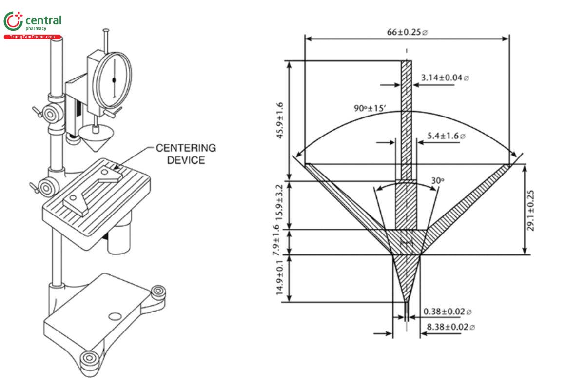
Briefly, the penetrometer cone positioned just above the surface of the semisolid is released and allowed to drop freely into the sample for 5 s. The penetration depth is recorded and reported in units of 0.1 mm. The penetration unit is decimillimeter (dmm). Three or more determinations are made, and the results are averaged to give the reported result. These penetrometry methods require the use of a two- piece cone (a small 30° cone attached to a larger 90° cone) that has a total effective mass of 150.0 ± 0.1 g. For this cone, gravity drives the cone into the semisolid with 1471 millinewtons (mN) of force.2 The effective penetration force (the total force minus the buoyancy force) results in the application of a shear stress to the semisolid at the surface of the penetrating cone. In general, the semisolid will respond to this applied shear stress according to the Herschel–Bulkley equation (Equation 3).

The cone will continue to penetrate until the applied shear stress is equal to the yield stress of the semisolid. At this point, the cone will stop penetrating and the shear rate will go to zero. It can be shown that, at this point, the yield stress will be a function of the penetration depth, h, according to Equation 11 below:

σ₀ = [cos²α/(π tanα)] × (1/h²) × [(W - (ρ_fgπh³ tan²α)/3]              Equation 11

where α is the half-angle of the cone, W is the weight of the penetrating cone, ρ is the density of the semisolid, and g is the acceleration from gravity. If the buoyancy correction is negligible, this equation simplifies as shown in Equation 12, indicating that the yield stress is essentially equal to the weight of the cone over the square of the penetration depth multiplied by a cone constant.

σ₀ = [cos²α/(π tanα)] × (W/h²)                  Equation 12

The term “hardness” (H) has been defined by several authors as shown in Equation 13,

H = C × (W/hⁿ)              Equation 13 

where C is a constant dependent on the cone geometry, W is the weight of the penetrating cone, h is the penetration depth, and n is an exponent. If n = 2, then H will be equivalent to the yield stress and have the same units (Pa).

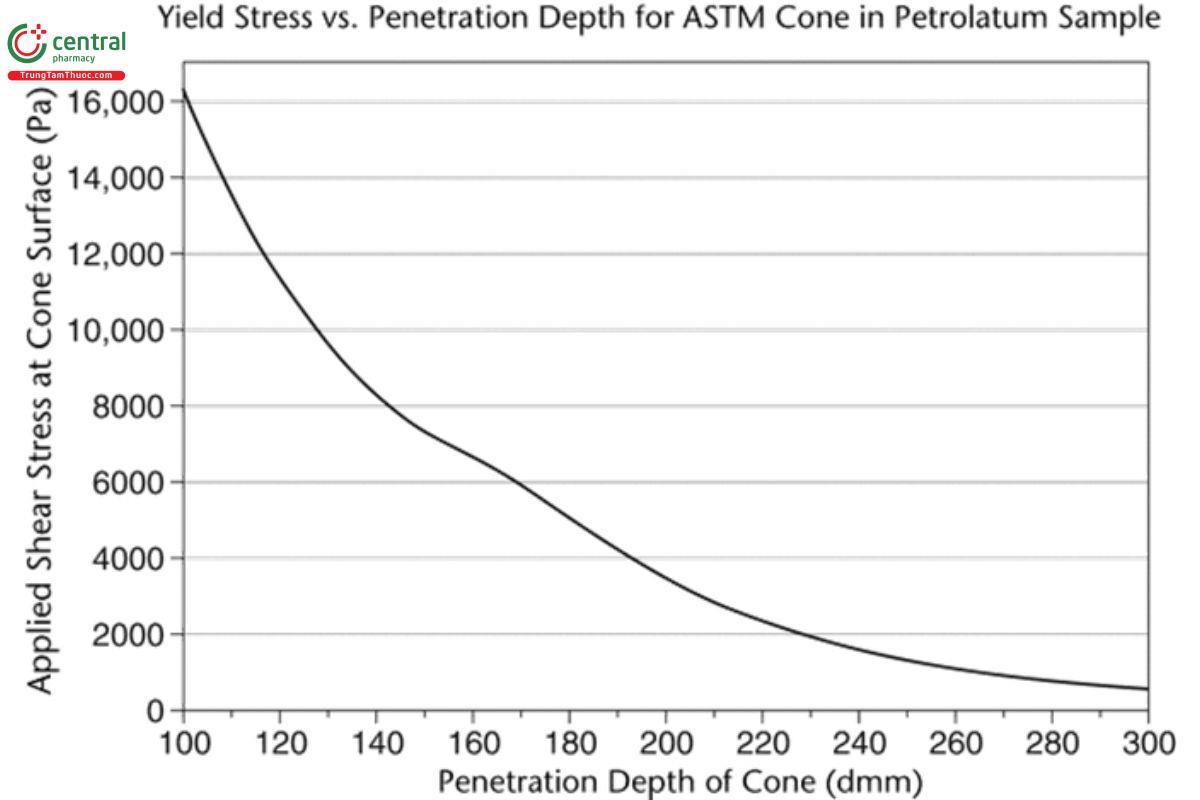
The monographs for petrolatum and white petrolatum each require the result of the penetrometry measurement to be in the 100–300- dmm range (NLT 10.0 mm and NMT 30.0 mm). Figure 6 shows the calculated yield stress for the standard 150-g, two-piece cone as a function of penetration depth.

3 GLOSSARY

Note that the following definitions are provided to clarify the use of these terms in the context of this chapter. These definitions are not intended to supersede or contradict definitions found elsewhere in USP–NF.

Consistency: See Structural strength.

Gel and Sol: A gel is defined as a material for which G′ > G″. A sol is defined as a material for which G′ < G″. The behavior of a gel is dominated by its elastic response to strain (shear deformation). The behavior of a sol is dominated by its viscous response to strain. The point where G′ = G″ is called the sol–gel transition. Rheology is used to characterize the continuous phase of a dosage form to classify it as either a gel or sol based on which behavior dominates the viscoelastic properties.

Hardness: Hardness is a term used synonymously with tensile stress, and yield stress is a type of tensile stress. Hardness is proportional with yield stress—a harder semisolid also exhibits a larger yield stress. In penetrometry, hardness has been more specifically defined as H = C × W/pⁿ, where C is a constant dependent on the cone geometry, W is the weight of the penetrating cone, p is the depth of penetration, and n is an exponent. When n = 2, hardness has the same units as yield stress (Pa).

Penetrometry: A method for quantifying the yield stress of semisolid materials in which a metal cone, with standardized dimensions and weight, penetrates into a semisolid until the buoyancy of the cone and the yield stress of the semisolid exactly balances the gravity-applied force driving the penetrating object into the semisolid. See  〈915〉 for more details.

Semisolids: Materials that exhibit viscoelastic properties that are classified as more solid-like at rest and at room temperature. Typically, these materials will transition to more fluid-like behavior under applied stress or as a result of temperature changes. This transition from a sol to a gel is identified as a yield stress. When used as dosage forms semisolids may be further classified as gels, ointments, or creams.

Strain: The shear deformation of a material. If a cubic volume of material is deformed by moving the top plane of the cube relative to the bottom plane of the cube, the strain is equal to the linear displacement of the top plane divided by the height of the cube (distance between the planes). This strain that results from the shear deformation of the viscoelastic material is unitless as it has units of distance (displacement) over distance. It is sometimes multiplied by 100 and reported as a percentage strain.

Structural strength (Consistency): Consistency is sometimes used synonymously with "viscosity", albeit incorrectly. Viscosity represents the proportionality of the shear stress to the shear rate for a Newtonian fluid, whereas consistency is the term for this proportionality for semisolids that exhibit non-Newtonian rheological behavior. Because the term consistency may be confused with uniformity or homogeneity, the term structural strength is now the preferred term.

Surface area: The surface area of the sheared fluid volume on which the shear force is acting or the cross-sectional area of material with area parallel to the applied force vector.

Wall slip: Term describing the shear-thinning of a semisolid dosage form at the wall of a measurement system. When shear stress is applied to a dosage form, the material at the wall of the measurement system will yield and shear thin before the remaining bulk material. This slipping of the material at the wall of the measurement system results in incomplete transfer of the shear stress into the bulk. Wall slip will result in erroneously low viscosity results for shear thinning and yield stress fluids and will result in erroneously high shear rate for a given applied shear stress. Wall slip is most significant for low shear measurements and can be reduced by using plate-plate measurement systems with roughened surfaces or by using a vaned rotor rather than a cylinder.

Yield stress: The applied stress at which a change in the viscoelastic properties of a semisolid is observed. Below the yield stress the material response is dominated by completely reversible elastic deformation, whereas above the yield stress, the material response is changing to irreversible elastic behavior (as the material remains a viscoelastic semisolid) or is dominated by viscous flow behavior.

4 REFERENCES

1. Zhang Q, Murawsky M, LaCount T, Hao J, Kasting GB, Newman B, Ghosh P, Raney SG, Li SK. Characterization of temperature profiles in skin and transdermal delivery system when exposed to temperature gradients in vivo and in vitro. Pharm Res. 2017;34(7):1491–1504.

2. US Food and Drug Administration. Guidance for industry. Transdermal and topical delivery systems—product development and quality considerations. 2019.

5 ADDITIONAL SOURCES OF INFORMATION

Larsson M, Duffy J. An overview of measurement techniques for determination of yield stress. Annu Trans Nordic Rheol Soc. 2013;21:125–138.

Barnes HA. The yield stress—a review or 'panta roi'—everything flows? J Non-Newtonian Fluid Mech. 1999;81:133–178.

Mezger TG. The Rheology Handbook: For Users of Rotational and Oscillatory Rheometers. Hanover: Vincentz, 2020 (5th ed).   Sun A, Gunasekaran S. Yield stress in foods: measurements and applications. Int J Food Prop. 2009;12(1):70–101.

Wright AJ, Scanlon MG, Hartel RW, Marangoni AG. Rheological properties of milkfat and butter. J Food Sci. 2001;66(8):1056–1071.   Deman JM. Consistency of fats: a review. J Am Oil Chem Soc. 1983;60(1):82–87.

Alderman NJ, Meeten GH, Sherwood JD. Vane rheometry of bentonite gels. J Non-Newtonian Fluid Mech. 1991;39:291–310.

ISO 3219-3: Rheology—Part 3: Test procedure and examples for the evaluation of results when using rotational and oscillatory rheometry.

Lin Y, Wang Y, Weng Z, Pan D, Chen J. Air bubbles play a role in shear thinning of non-colloidal suspensions. Phys Fluids. 2021;33:011702.

(USP 1-Dec-2023)