ANALYTICAL METHODOLOGIES BASED ON SCATTERING PHENOMENA—SMALL ANGLE X-RAY SCATTERING AND SMALL ANGLE NEUTRON SCATTERING
If you find any inaccurate information, please let us know by providing your feedback here

Tóm tắt nội dung
This article is compiled based on the United States Pharmacopeia (USP) – 2025 Edition
Issued and maintained by the United States Pharmacopeial Convention (USP)
INTRODUCTION
Small-angle X-ray scattering (SAXS) and small-angle neutron scattering (SANS) make up a sub-family of small-angle scattering (SAS) diffraction techniques suitable for probing the size, shape, ordering, and interactions of molecules and molecular assemblies on length scales that are typically from around 1 nanometer, to a few hundred nm. This size range overlaps with the lower range probed using the laser light diffraction technique (see Analytical Methodologies Based on Scattering Phenomena—Light Diffraction Measurements of Particle Size 〈1430.2〉).
Because these length scales are much larger than inter-atomic distances, in crystallographic terms SAS is considered low-resolution diffraction. Nonetheless, it is an extremely useful and versatile technique capable of providing structural information complementary to cryogenic transmission electron microscopy (cryo-TEM), high-resolution nuclear magnetic resonance (NMR), and analytical ultracentrifugation.
SAS differs from dynamic light scattering (DLS; see Analytical Methodologies Based on Scattering Phenomena—Dynamic Light Scattering 〈1430.3〉) in that it is a direct probe of size and shape.
1.1 Applications
SAS is routinely performed on solids, liquids, and dispersion samples (both aqueous and nonaqueous). Some types of SAS have been used to study foams.
In terms of pharmaceutical applications, SAS has been used to study topical creams, intravenous emulsions, hydrogels, polymer-drug conjugates, proteins, enzymes, and antibodies (1–5). Some types of SAS are particularly well suited to studying the physical chemistry underlying formulation problems.
SAS can be used in various applications to evaluate the size, shape, and ordering of molecules. For example, SAS can provide information on the size and dispersity of droplets, macromolecules, micelles, liposomes, nanoparticles, crystalline domains, and pores (including in mixtures of these and other multi-phase systems). With regard to shape, SAS can be used to determine the shape of micelles and nanoparticles; the tertiary structure of proteins, enzymes, and antibodies (using SAS-constrained modeling); and the conformational distribution of adsorbed layers. Finally, examples of the use of SAS to assess molecular order include determining the core-shell structure of micelles and sterically stabilized nanoparticles, the bilayer structure in liposomes, and the liquid crystalline structure (e.g., lattice parameters, space groups).
TYPES OF SAS
SAS is a specialized, but nonetheless highly useful and versatile, technique. Although a detailed discussion of SAS is beyond the scope of this chapter, the intention of this chapter is to raise awareness and then direct the reader to authoritative sources for further information.
SAS is most commonly performed using light [small-angle light scattering (SALS)], X-rays (SAXS), or neutrons (SANS). It is the wavelength of these different radiation sources, and the way that the radiation interacts with the atoms in a sample, that determines what type of information is obtained in a particular SAS experiment. Importantly, data from all of these variants of SAS can be analyzed using common formulae and software packages. Table 1 summarizes some of the key aspects of the different types of SAS.
Table 1. Key Aspects of Different Types of Small-Angle Scattering
| Parameter | SALS | Lab-SAXS | Synchrotron-SAXSᵃ | SANSᵃ |
|---|---|---|---|---|
| Radiation scattered by | Electrons | Electrons | Electrons | Nuclei |
| Radiation velocity (m/s) | 3 × 10⁸ | 3 × 10⁸ | 3 × 10⁸ | 10²–10³ |
| Accessibility | Laboratory | Laboratory | Synchrotron source | Neutron source |
| Relative brilliance | Medium | Medium | High | Low |
| Wavelengths (nm) | 400–700 | 0.07–0.23 | 0.06–0.33 | 0.15–2.5 |
| Length scales probed (nm) | 250–25,000 | <1–350 | 0.1–2500 | 0.2–1000+ |
| Impact of dust contamination | Significant | Negligible | Negligible | Negligible |
| Effect of hydrogen (H)/deuterium (D) substitution | None | None | None | Large |
| Radiation/heat damage | Negligible | Possible | Very likely | Negligible |
| Absolute intensity calibration | Possible | Possible | Possible | Routine |
| Sample volumes (mL) | 0.05–5 | 0.007–0.1 | 0.0001–0.5 | 0.1–5.5 |
| Study optically opaque samples | No | Yes | Yes | Yes |
| Typical container materials | Glass, quartz | Polyimide (Kapton), polycarbonate, beryllium, silica/quartz, silicon nitride | Polyimide (Kapton), polycarbonate, beryllium, silica/quartz, silicon nitride | Silicon, silica/quartz, aluminum, titanium, vanadium, copper silicon nitride |
ᵃ Access to national and international large facilities is usually obtained through competitive peer review, but experimental time for successful proposals is then free, provided that the results are placed in the public domain. Where this route of access is unsuitable, for example, for commercial customers who require confidentiality or a guarantee of experimental time, a range of paid industrial access mechanisms will typically be available.
1 BASIC THEORY
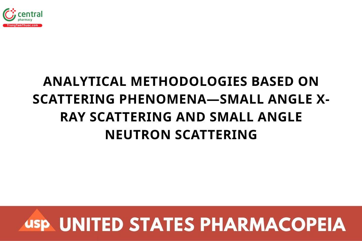
When a beam of radiation is directed at a sample, a fraction of the beam will be transmitted, a fraction will be absorbed (and in some experiments may then be re-radiated), and the remainder will be diffracted through a range of angles, θ. In a typical SAS experiment, 0.01° < θ < 10°; this value of θ is different from that in wide-angle and classical crystallographic diffraction experiments, where θ > 10°. On some instruments, it may be possible to record the small- and wide-angle data concurrently.
Radiation scattered through the same angle but originating from different points in the sample may then superimpose constructively or destructively at the detector to construct a “scattering pattern”. This reflects spatial fluctuations in the refractive index (RI) (SALS), electron density (SAXS), or scattering length density (SANS) of the sample, which in turn arise from differences in the size, shape, and order of the constituent molecules.
The length scale, d, of the spatial fluctuations that may be accessed in a SAS experiment is determined by Bragg’s Law:
d = λ / (2 sin(θ))
where λ is the wavelength. Experimentally, it is more typical to express this in terms of (the modulus of) a quantity called the “scattering vector”, q:
q = (4π/λ) sin(θ) = |q| = |k_s − k_i|
from which it follows that:
d = 2πn / q
where k_i and k_s are the incident and scattered wave vectors and n is the RI of the medium. Conveniently, for neutrons and for X-rays, n may be assumed to be unity. Note that q is an inverse length scale. The geometry of a SAS experiment is illustrated in Figure 1.
The number of photons/neutrons of a given wavelength, scattered through a particular angle, that arrive at a detector pixel in a unit time, N(λ,q), may be expressed as:
N(λ,q) = N₀(λ)ΔΩ η(λ)T_r(λ)V_s I(q)
where N₀ is the incident flux of photons/neutrons, ΔΩ is the solid angle element defined by the size and distance of the detector pixel from the sample, η is the detector efficiency, T_r is the transmission of the sample (i.e., 1 − absorbance), V_s is the volume of the sample illuminated by the beam, and I(q) is the scattering function. Note that the first three terms are instrument-specific, whereas the last three terms are sample-dependent. The scattering function, the quantity determined in an SAS experiment, is given by:
I(q) = ΦV(Δρ)²P(q)S(q) + B
where Φ is the volume fraction of the scattering objects in the sample (e.g., the volume fraction of nanoparticles in a dispersion); V is the volume of one scattering object; Δρ = (ρ_object − ρ_matrix) is the contrast of the sample (discussed below); the form factor P(q) describes how the scattering is modulated by the size, shape, and dispersity of the scattering objects; the structure factor S(q) describes how the scattering is modulated by interactions; and B is a residual background signal normally taken to be q-independent. P(q) has a value between 0 and 1. As Φ → 0, so S(q) → 1.
For a solute in solution:
ΦV = cM / (N_A δ²)
where c is the mass concentration of the solute, M is its formula weight, and δ is its bulk density. The objective of an SAS experiment is to extract information from P(q) and/or S(q). How this is achieved is discussed later. However, every component in the sample, including the container, will contribute to the overall scattering from the sample. So in addition to obvious background correction measurements (e.g., empty container; container + solvent), it is often useful to manipulate the various other individual contributions.
2 CONTRAST MATCHING
From the discussion in the preceding section, it is apparent that if the contrast term is zero, there will be no SAS. This condition is known as “contrast matching” and is potentially extremely useful because it permits the simplification of the scattering from complex multi-component samples and the study of individual components.
In SALS, contrast matching requires that two or more components have the same RI. The reader may have experienced this phenomenon when washing a glass in a bowl of water; the glass can seem to disappear because the glass and the water have similar RIs. In many experiments, however, RI matching of the components in a sample is often difficult to achieve in a useful manner. Some SALS and DLS instruments, however, use index-matching baths around the sample cell to reduce scattering from the outer wall of the cell.
In SAXS, contrast matching requires that two or more components have the same electron density. Because the electron density of a molecule is strongly influenced by the atomic number of the elements it contains, contrast matching a molecule with a heavy atom, such as a cationic surfactant, to an aqueous medium is not possible unless an additional solute is added to bolster the electron density of the medium. However, this course of action may change the pristine characteristics of the analyte and its chemical environment.
Contrast matching is more useful in SANS. Here, contrast matching is achieved if two or more components have the same scattering length density, ρ:
ρ = (δN_A / M) Σ b_j
where b_j is the (bound) “coherent neutron scattering length” of nucleus j, and the other variables are as defined previously. The summation only needs to be performed over the empirical formula for a component.
Scattering length density calculators can be found online or as tools in some SAS analysis programs. A compendium of neutron scattering lengths is available online (6).
An example of a calculation for poly(ethylene oxide), –[CH₂–CH₂–O]–ₙ:
C₂H₄O, M = 44 g/mol, δ = 1.127 g/cm³, b in cm
ρ = (1.127 × 6.023 × 10²³ / 44) × {(2 × 6.646 × 10⁻¹³) + (4 × −3.739 × 10⁻¹³) + 5.803 × 10⁻¹³}
ρ = 0.64 × 10¹⁰ cm⁻² or 0.64 × 10⁻⁶ Å⁻²
Importantly, because they depend on the neutron-nucleus interaction, scattering lengths are isotope-dependent. The same calculation for perdeuterated poly(ethylene oxide), for example, would yield ρ = 6.46 × 10¹⁰ cm⁻².
[NOTE—It is a coincidence that this value appears to be 10 times the hydrogenous value.]
Thus, D-for-H exchange offers significant opportunities for exploiting contrast matching in soft-matter SANS experiments.
Table 2 lists some illustrative scattering length densities. These may sometimes be found expressed in the equivalent but non-SI units of 10⁻⁶ Å⁻².
Table 2. Neutron Scattering Length Densities of Pharmaceutically Relevant Molecules
| Molecule | ρ (10¹⁰ cm⁻²) | Molecule | ρ (10¹⁰ cm⁻²) | Molecule | ρ (10¹⁰ cm⁻²) |
|---|---|---|---|---|---|
| H₂O | −0.56 | H₂₅–sodium dodecyl sulfate (SDS) | 0.33 | Lipids | 0.1–0.4 |
| D₂O | 6.37 | D₂₅–SDS | 5.83 | Proteins | 2.2–2.6 |
| H₈–toluene | 0.94 | H₆₀–Triton ×100 | 0.57 | Carbohydrates | 2.7 |
| D₈–toluene | 5.66 | H₃₁–dodecyldimethylamine oxide (DDAO) | −0.20 | DNA | 4.0 |
| Perfluorodecalin | 4.21 | H₃₉–deoxycholate Na | 0.66 | RNA | 4.5 |
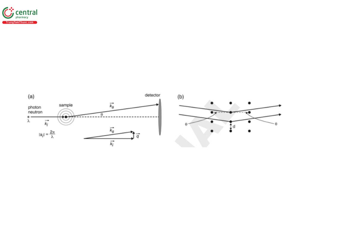
Several useful characteristics of scattering length densities are evident in the table. First, they can be positive, negative, or, in principle, zero. Second, different classes of biological molecules span a wide range of scattering length densities. Lastly, it is usually possible to find a solvent, or preferably a mixture of solvents, that will contrast match any solute. So, for example, DNA can be contrast matched in a mixture of 34.1% H₂O:65.9% D₂O by volume, and a perfluorodecalin-in-water emulsion would not scatter neutrons if the oil was dispersed in a mixture of 31.1% H₂O:68.9% D₂O by volume. It is even possible to make an H₂O:D₂O mixture that does not scatter (i.e., Δρ = 0). Figure 2 shows how contrast matching could be used in a SANS study.
When calculating scattering length densities, it is important to use as accurate a value as possible for the bulk density, δ. However, sometimes determining δ can be problematic for deuterated compounds. In such instances, a useful rule of thumb for solvents and relatively simple molecules is δ_D = δ_H × 1.1. Also, it is important to remember that δ is temperature-dependent.
Molecules containing hydroxyl groups, carboxylic acid groups, and even some amine groups will readily exchange those functional protons for deuterons when exposed to D₂O. This means that the scattering length density of some molecules can be pH-dependent; proteins are an obvious example. Some scattering length density calculators include a degree of exchange parameter to compensate for this pH dependence.
3 INSTRUMENTATION
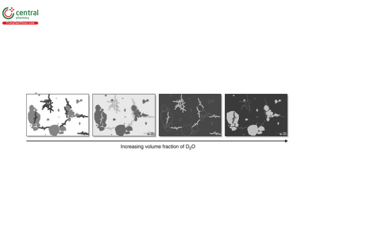
The components of a SAS system (see Figure 3) are common across the different forms of the technique.
Key
Source
Optics
Slits
Sample
Detector
SALS and SAXS are performed using monochromatic radiation, which is collimated with slits or pinholes to the desired profile regarding size (diameter or width/height) and shape (line or point). The wavelength of monochromatic radiation is determined by the choice of source (replacing one type of anode material with another), but may also be varied by changing optical filters, or adjusting the synchrotron monochromator. SANS at reactor neutron sources is also performed in this manner, with the wavelength adjustment performed by a rotating device called a velocity selector. In these fixed-wavelength measurements, altering the dynamic range in q of the instrument requires changing the sample-to-detector distance (either along the incident beam direction or off-axis) in order to change the range of scattering angles subtended to the sample.
However, SANS can also be performed at pulsed neutron sources (based on particle accelerators—so-called spallation sources—or pulsed reactors). At these sources, a “polychromatic” (“white”) beam of neutrons is directed at the sample, and the time of flight (TOF) of the scattered neutrons to the detector is recorded. This establishes the neutron velocity and thereby its wavelength. The dynamic range in q of these TOF-SANS instruments is much broader than that of their fixed-wavelength counterparts because every wavelength that reaches a pixel on the detector corresponds to a different q value, although a given pixel on the detector still represents a single scattering angle. Moreover, the intrinsic wavelength resolution, and therefore q-resolution, of TOF-SANS is much better than that of fixed-wavelength SANS.
The scattering from a sample actually occurs over 4π space, but because an SAS instrument is linear, the detector only intercepts a conic section of the total scattering. Because most soft matter samples have some degree of intrinsic disorder (referred to as “polycrystallinity” by crystallographers), the detector records multiple rings of varying intensity rather than discrete spots (reflections) see Figure 4.
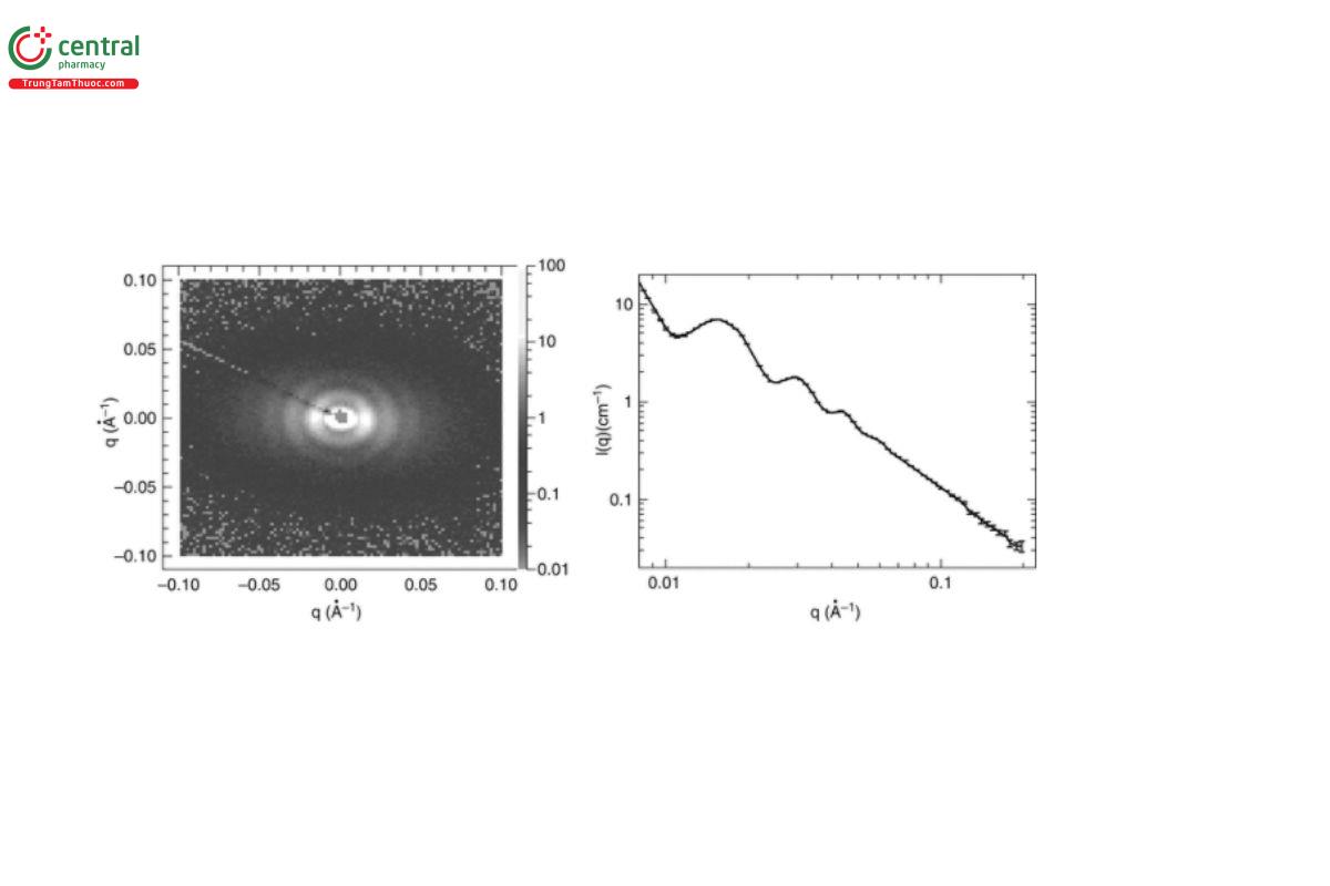
The scattered radiation will usually be detected by solid-state charge-coupled device (CCD) cameras (SALS/SAXS), gas detectors (SAXS/SANS), or scintillator detectors (SANS). Often these will be highly pixelated two-dimensional (“area”) detectors, which are extremely useful for resolving anisotropic scattering from oriented samples. A state-of-the-art SAXS detector for laboratory applications may have 1 thousand (for one-dimensional detectors) to more than 1 million pixels (for two-dimensional detectors), and more for large-facility instruments. Consequently, the data volumes generated during an experiment may be quite large (gigabytes to terabytes).
In order to allow them to access smaller angles, and because they require more substantial radiation shielding, SAXS/SANS instruments at large facilities may extend several tens of meters from the source. Even a state-of-the-art laboratory SAXS instrument is typically 3–5 m in length. While in principle one could attain ever-smaller q values by building very long instruments, in practice the count rate at the detector declines as the inverse-square of the sample–detector distance; thus, measurements become impractically slow. To circumvent this limitation and permit very-small-angle scattering (VSAXS/VSANS) or ultra-small-angle scattering (USAXS/USANS) measurements, alternative strategies are employed, such as using focusing optics or slit-collimated Bonse–Hart “double-crystal” geometries. These instruments can access length scales (d) into the micron scale, i.e., the same realm accessible by optical microscopy. The type of source collimation, point-source (pinhole) versus slit, has implications for data processing. Very recently, a new form of SANS has emerged wherein the scattering angle is encoded in the precision of polarized neutrons. This technique, spin-echo (modulated) SANS (SESANS/SEMSANS), can also access micron-length scales but measures in d-space rather than in q-space. Its advantages over Bonse–Hart VSANS are that it retains good count rates and is much less susceptible to multiple scattering from the sample. Further discussion of these extended SAS techniques is beyond the scope of this chapter, but the reader should be aware of their existence.
Change to read:
4 EXPERIMENTAL CONSIDERATIONS
Performing a successful SAS experiment depends on many factors, including but not limited to the following factors described in subsections 6.1–6.12 (7–9).
6.1 Incident Flux
Incident flux is the number of photons/neutrons per unit area per second delivered to the sample. It is a function of the brilliance of the source (see Table 1) and the wavelength selection/collimation employed for the experiment. Kinetic or dynamic measurements, or measurements on very weakly scattering samples, will fare better on higher-flux instruments.
6.2 Resolution
There are two types of resolution of relevance to an SAS experiment:
Size resolution of the instrument
q-resolution of the measurement
6.2.1 SIZE RESOLUTION
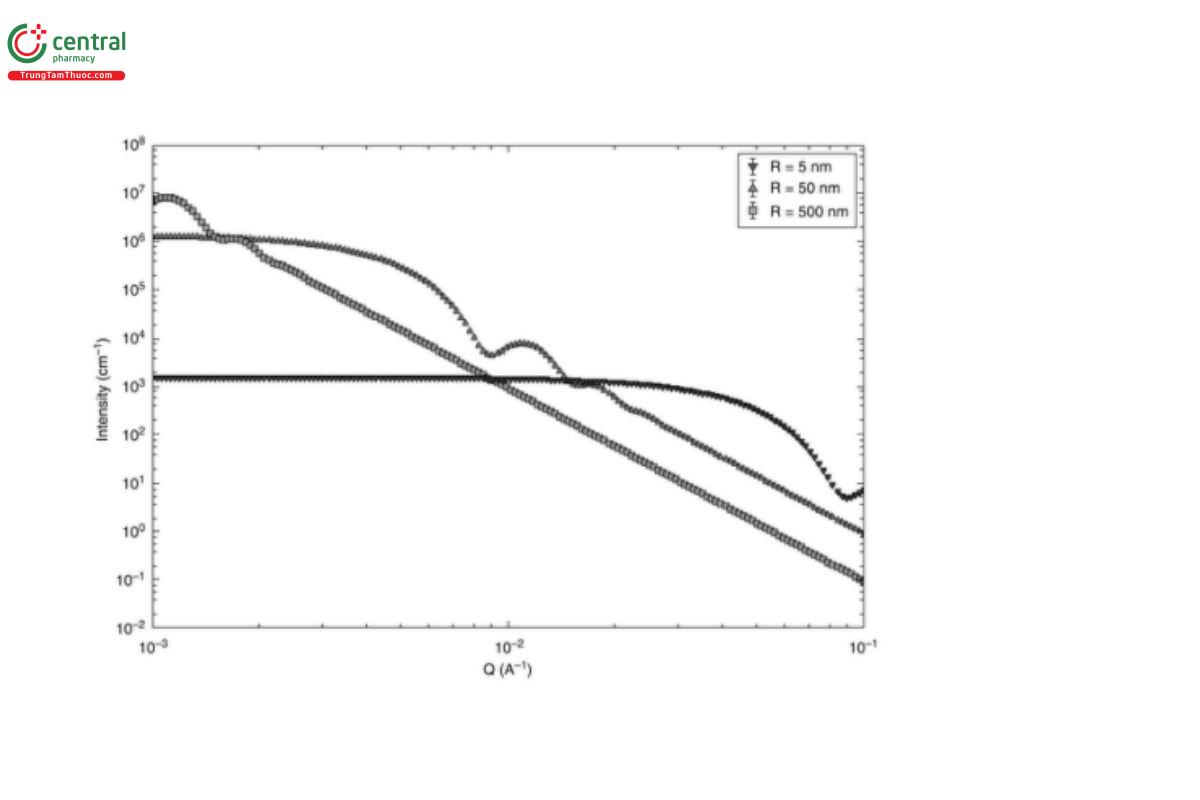
The maximum, d_max, and minimum, d_min, length scales of the structure to be probed need to lie inside the measurement limits of the instrument, i.e.:
q_min < π / d_max ▲ (ERR 1-Dec-2019)
and
q_max > π / d_min
This principle is illustrated in Figure 5.
6.2.2 q-RESOLUTION
The q-resolution is the precision with which adjacent q-points can be distinguished, and therefore it governs the level of fine detail in the measured scattering data that can be resolved (for example, the peaks in Figure 4).
The q-resolution is primarily determined by the wavelength resolution of the instrument, then by the geometric resolution arising from the selected instrument collimation, and then by a range of other less significant factors.
Laser light sources and X-ray sources offer the best wavelength resolution, with Δλ/λ values as low as 0.01%. Conventional light sources depend on the use of a bandpass filter for which Δλ/λ may be ~1%. Although good wavelength resolution is an intrinsic property of a laser, in the case of X-rays, it is determined by the monochromator in use. The wavelength resolution of fixed-wavelength SANS instruments depends on the specification of the neutron velocity selector employed. Typically, this resolution will be between 8% and 20%. However, in TOF-SANS the wavelength resolution is determined by the precision with which the neutron TOF (typically a few thousand microseconds) can be measured, and thus Δλ/λ values of approximately 5% would not be uncommon. In most instances, better wavelength resolution can always be traded for reduced flux and vice versa.
The geometric resolution is essentially governed by the beam size at the sample; a smaller size is better. Laser-based SALS and SAXS instruments with submillimeter beam footprints fare much better than SANS instruments in this regard, where a relatively small beam may still be 6–8 mm in diameter. This difference is further compounded by the fact that because neutrons cannot be easily focused, reducing the beam footprint also decreases the flux on the sample.
6.3 Instrument Calibration
SAS instruments require two separate calibrations, but with an astute choice of calibration sample it might be possible to perform both calibrations in one measurement:
Calibration of the q-scale
Calibration of the intensity scale
An instrument technician or, at large facilities, the assigned experiment local contact, will normally perform these calibrations. However, if one’s plan is to use several different SAS instruments it is advisable to acquire and measure one’s own calibrants to ensure confidence in the local calibrations and ensure that all of one’s data are on self-consistent scales.
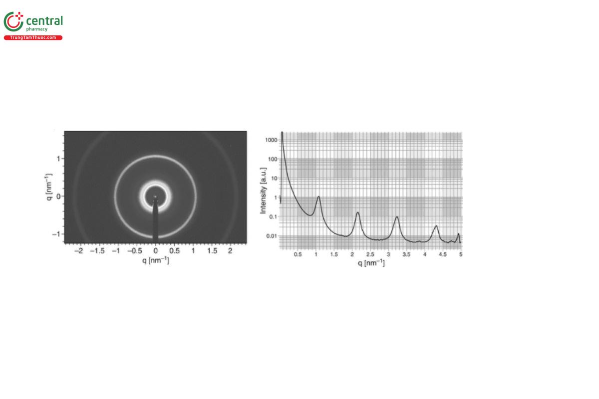
6.3.1 q-CALIBRATION
It is possible to omit the q-calibration on a fixed-geometry SAS instrument where the sample-to-detector distance is constant/known. In all other instances, it is necessary to measure a sample with a characteristic q-dependence related to structure that can be unambiguously verified by other means (e.g., TEM, atomic force microscopy (AFM), etc.). Alternatively, if an SAXS instrument has an energy-responsive detector, and an accurate determination of scattering angle is possible, then an absorption edge can be used to verify q. Two commonly used q-calibrants for SAXS/SANS are silver behenate (AgBh) (see Figure 6) and rat tail Collagen (RTC).
6.3.2 INTENSITY CALIBRATION
Intensity calibration relies on the fact that for some types of material, I(q = 0) can be related to molecular parameters that can be calculated with reliability or determined using other techniques, for example, the molecular weight of a polymer, the surface area-to-volume ratio of a porous solid, or the second virial coefficient or isothermal compressibility of a pure liquid. However, because an SAS instrument does not physically collect data at q = 0, an extrapolation is required. Extrapolation is only possible, with the necessary precision, if the scattering function for the chosen calibrant has a definitive form. Commonly used intensity calibrants include water (SAXS; 10), Lupolen (SAXS), blends of hydrogenated and perdeuterated homopolymers (SANS; 11,18), porous solids (SAXS/SANS; 18), glassy (vitreous) carbon (SAXS/SANS; 12,18), and vanadium (SANS).
6.4 Sample Quality
As in any experiment, the best results will be obtained using carefully prepared samples. In particular, because the SAS from an object scales as the sixth power of its size, the presence of even a relatively few large objects in a sample can disproportionately interfere with the quality of the data, all else being equal. SALS is particularly affected by the presence of large particles because of the aforementioned difficulties in RI matching. For this reason, solvents used for SALS experiments should be rigorously filtered before use to exclude the presence of dust particles. SAXS and SANS (but not USAXS/USANS) are much less affected by dust because they probe shorter length scales (dust particles are micron-sized). However, the presence of unwanted, unintended, or unexpected aggregation of components of the sample can be just as troublesome. Prescreening for aggregation in biological samples destined for SAXS or SANS instruments (for example, by DLS) should be considered de rigour. Poor contrast in a sample can also be problematic, although in some instances (for example, in SANS contrast matching experiments), it is unavoidable.
6.5 Sample Concentration
Although the magnitude of I(q), and the precision with which it is measured, are both generally improved by using more concentrated samples, this comes with disadvantages as well, i.e., lower transmissions (see 6.9 Sample Transmission) and the possible introduction of atomic pair correlations manifesting themselves in an S(q) contribution to the scattering function. Whether this is an issue depends on the sample being studied and the intended method of data analysis. Some relatively simple modeling of the scattering before the experiment may help to establish the viable concentration envelope.
Of course, the converse is also true, and very dilute samples will likely suffer from a poor signal-to-noise ratio and necessitate longer experimental counting times, although this longer experimental time might be mitigated by the use of a high-flux instrument. However, as an illustration, most SAXS/SANS instruments can handle protein/enzyme solutions at concentrations as low as Φ ~ 0.1% (1 mg/mL), whereas S(q) is not usually a concern in a colloidal dispersion at Φ > 5%. For investigations of S(q), relevantly higher concentrations are used.
6.6 Sample Containers
Unless one is working with a self-supporting sample, the sample will need to be contained. The problem with sample containers is that they also scatter, so the material from which they are constructed is an important consideration. Suitable container window materials combine the mechanical strength and chemical resistance with high transmittance and scattering features, which do not interfere with those of the sample. As such, multiple window materials may be necessary to cover the entire range over which a sample is to be measured.
For SALS and SAXS, it is quite common to use glass sample containers. Glass is composed only of light atoms (an important consideration for SAXS), and its transparency is useful for observing the sample as it is a prerequisite for SALS. However, because glass contains boron (a neutron absorber) it is not suitable for SANS.
Amorphous synthetic quartz (SiO₂, also called fused silica) is a good choice of material for SALS, SAXS, and SANS. It can be cut, polished, and fabricated and is also transparent and only composed of light atoms; however, it is boron-free. It also has good thermo-mechanical stability over an experimentally useful range of temperatures and is chemically inert to all but concentrated bases and hydrofluoric acid. Material tradenames include Spectrosil and Suprasil, but in principle anything suitable for far-UV (not IR) spectrophotometry should suffice.
For SAXS, it is possible to utilize sample containers constructed from amorphous engineering polymers such as poly(carbonate) (PC), poly(etheretherketone) (PEEK), or poly(imide) (Kapton). Poly(amides) (nylons) are not suitable because they are semi-crystalline. All hydrogenous polymers are wholly unsuitable for use as SANS sample containers.
The greater penetrating ability of neutrons means that SANS sample containers can be constructed from metals. Pure metals should be used where possible (as SANS is an excellent technique for probing the nanostructure of metal alloys), or when a prior assessment of suitability has been conducted. Good choices of metals for use with neutrons are aluminum, titanium, vanadium, and copper. These metals
can activate on prolonged exposure to neutron radiation but not to levels that make them impractical to use. Beryllium, being of low atomic number, is however a practical choice for SAXS.
In most experiments, the sample will simply be contained in the quiescent state in a capillary or cuvette. However, it is important to understand that quiescent conditions are not necessary. Indeed, the ability of SAS to probe a sample under changing conditions (pH, temperature, pressure) or applied fields (electric, magnetic, shear) is usually where the greatest information is ultimately derived. The use of cryostats, furnaces, pressure cells, rheometers, tensile stages, and stop-flow cells with SAXS/SANS instruments is very common. The use of flow-through cells to mitigate radiation damage (see 6.11 Radiation Damage) is very common on high-flux SAXS instruments.
Sample containers will typically have path lengths ranging from 0.1–2 mm (SAXS) to 1–5 mm (SANS) to 10 mm or more (SALS). Multiplying this value by the incident beam size—a few micrometers (SAXS) to a few millimeters (SALS/SANS)—reveals that the required sample volume is rarely more than a couple of milliliters, and potentially less.
6.7 Backgrounds
In the same way that the sample container contributes to the measured scattering, so does the matrix containing the sample, for example, the dispersion medium. For this reason, it is typical to measure the scattering from the pure matrix, in the same or an identical sample container under the same experimental conditions, and then to subtract this matrix scattering from the sample scattering. This procedure should also correct for other sources of “sample-independent” background (for example, the container, vacuum windows, detector response, etc.).
Difficulties can arise if the sample component of interest occupies a substantial proportion of the overall sample volume because subtracting 100% of the matrix may no longer be appropriate, leading to over-correction of the data. In these instances, a volume fraction-weighted background correction may be appropriate.
Arguably, the most insidious form of “sample-independent” background is multiple scattering (discussed in 6.10 Multiple Scattering).
6.8 Counting Times
Experimental measuring times for an SAS experiment may vary from a fraction of a second (synchrotron-SAXS) to many minutes or hours (SANS). However, because SAS measurements are Poisson counting processes, to halve the statistical uncertainty on an I(q) point requires four times as much data. This calculation is further complicated by the fact that when a background is subtracted, the statistical errors on the sample and backgrounds are added in quadrature, as shown here:
Error_sample−background = √{ (Error_sample)² + (Error_matrix)² }
Thus the final data quality may not be apparent until after the experiment has finished. This means that invariably one ends up making a judgment call about the statistical quality of the data before moving on to the next sample. Therefore, counting times are often based on previous experience or simple trial-and-error, or a combination of both. A good rule of thumb is to measure each background for the same number of photons/neutrons as the sample it is intended to correct.
6.9 Sample Transmission
The sample transmission, T_r, is a dimensionless number ranging between 0 and 1 and is a measure of the balance between the scattering power of the sample and absorption as described by the Beer–Lambert Law:
T_r = exp(−μt) = 1 − A
where t is the pathlength (in most instances, the thickness) of the sample, μ is an absorption coefficient, and A is the absorbance; μ is dependent on the type of radiation in use.
Despite the simple appearance of this expression, accurately calculating T_r for a sample is fraught with difficulties because μ may be unknown or difficult to determine. The best course of action is to measure T_r at the time the SAS is recorded, simultaneously, if possible.
Note that in TOF-SANS, T_r is a function of wavelength.
A good rule of thumb is to keep T_r > 0.37 (i.e., t < 1/μ), although this will have consequences for multiple scattering (see 6.10 Multiple Scattering).
6.10 Multiple Scattering
Multiple scattering is where a photon/neutron that has been scattered once by the sample is scattered again (possibly several times). Multiple scattering should be avoided, if possible, because a routine method for correcting SAS data for multiple scattering has not been developed, except in some limited circumstances. The essence of the problem is that the history of multiply scattered photons/neutrons is unknown, and thus one cannot know whether or not to use them.
It is, however, quite straightforward to estimate the extent of multiple scattering from a sample. To a first approximation, the average number of times a photon/neutron has been scattered, τ, is:
τ = μt = −ln T_r ∝ t²
Thus, even for T_r = 0.9 there is a 10% probability of multiple scattering. By T_r = 0.5 that probability has risen to almost 70%.
If multiple scattering is suspected, two strategies for mitigating its effects are to thin the sample and/or use shorter wavelengths and then re-measure and look for differences.
6.11 Radiation Damage
An important consideration during SAXS, particularly synchrotron-SAXS, experiments is that the X-ray beam can be extremely destructive to some samples if mitigating strategies are not deployed, such as the use of flow-through cells or cryogenic cooling. This is because the energy of the X-ray photons [for example, 8047 eV at the copper (Cu) Kα wavelength of 0.154 nm] is far greater than the strength of the bonds holding the sample together (for example, the C–C bond energy is just 4 eV), and hydrogen bonds are weaker still. Even visible photons from a modest blue laser can cause sample degradation if left to irradiate the sample for long enough. Conversely, the energy of neutrons of equivalent wavelengths are orders of magnitude lower (for example, a mere 0.034 eV at a wavelength of 0.154 nm), meaning neutrons are a truly non-destructive probe, especially of sensitive biological material.
6.12 Sample Deuteration
Although selective deuteration is a valuable experimental tool for extracting maximum information from a SANS experiment, it is unfortunately not without complications. The slightly larger atomic volume of deuterium, differences in the polarizability of C–H bonds and C–D bonds, and differences in the strength of O...H and O...D hydrogen bonds all contribute to subtle modifications of the underlying thermodynamics in the sample which can, and do, affect the phase behavior. For example, cloud points, critical micelle concentration, micelle aggregation numbers, and theta temperatures have all been known to change (sometimes in opposite directions depending on whether the solute or the solvent is deuterated). These challenges should be considered when designing a SANS experiment.
5 DATA PROCESSING
SAS data processing has two steps:
Data reduction: The transformation of the as-measured instrument-dependent data into portable instrument-independent data (ideally in absolute units on an absolute scale)
Data analysis: The interpretation of the instrument-independent data to extract physical information characterizing the sample
7.1 Data Reduction
Data reduction procedures, and the factors for which they are corrected, will vary from one SAS instrument to the next. In the case of SANS, these procedures can even vary between reactor-SANS instruments and TOF-SANS instruments. However, every SAS instrument manufacturer or large facility will provide the necessary software to correctly reduce the data collected from their instrument(s). This software is typically graphical user interface (GUI)-driven (although scripts are still used) and will offer both “novice” and “expert” modes of use, for either “manual”/“single” or “automated”/“batch” data reductions.
In general, the data reduction process will include most or all of the following steps:
Correct for the detector efficiency, dark current, dead time, and spatial linearity (flatness)
Calculate the q values of each detector pixel
Integrate the recorded counts at a given q within some region of interest (azimuthal angle, sector, etc.)
Normalize for the incident flux or quantum efficiency of the source
Correct for the sample transmission (absorbance correction)
Correct for the volume of sample illuminated (beam area × sample thickness)
Apply an intensity calibration factor
Convert the intensity scale into absolute units
This process is repeated for every sample measured, and for any backgrounds measured. The appropriate background is then subtracted from a sample to yield the final, fully reduced SAS data set.
7.2 Data Analysis
SAS data analysis for a single sample may use one or more of the following methodologies:
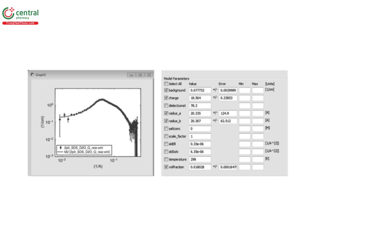
• Model-fitting/curve-fitting methods:
○ Involve optimized fitting of analytical functions for P(q) and/or S(q) to the experimental I(q) data, for example, to determine generic shape information (sphere, cylinder, coil, etc.), size (radius, radius-of-gyration, cross-sectional radius, etc.), and interaction potentials (hard sphere, Percus–Yervick, etc.) (see Figure 7)
○ Applicable to all sample types
○ Computationally straightforward
• Real-space methods:
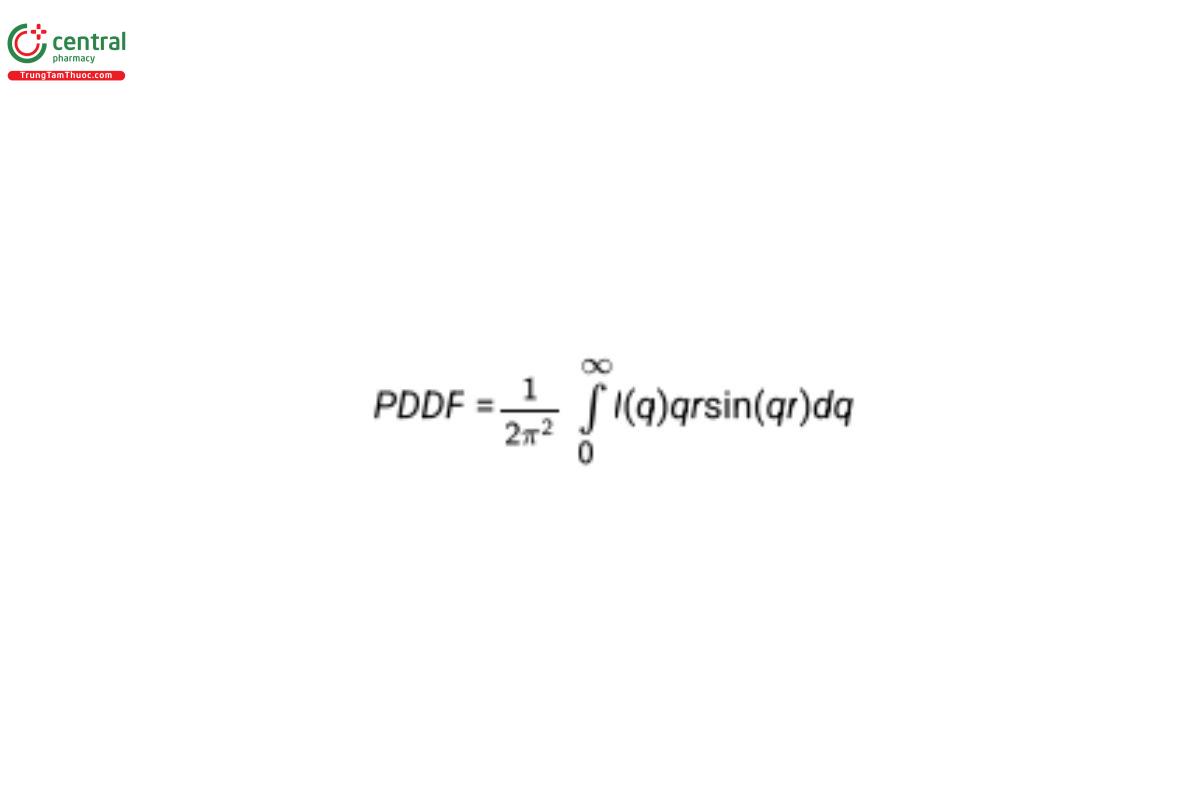
○ Involve mathematical transformation of the experimental I(q) data from reciprocal-space to real-space, for example, to obtain density correlation functions (Γ(r)), distance distribution functions [pair-distance distribution function (PDDF) or P(r)], or scattering length/segment density profiles [ρ(r)] (see Figure 8)
○ Applicable to all sample types
○ Computationally straightforward
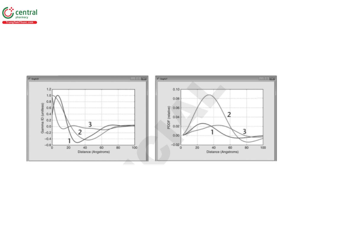
Γ(r) depicts the average separation of regions of similar scattering-length density in the sample. The minima and maxima in the function represent structural boundaries, for example, the edge of the object:

where the “scattering invariant” (also called the “total scattering”) is given by:
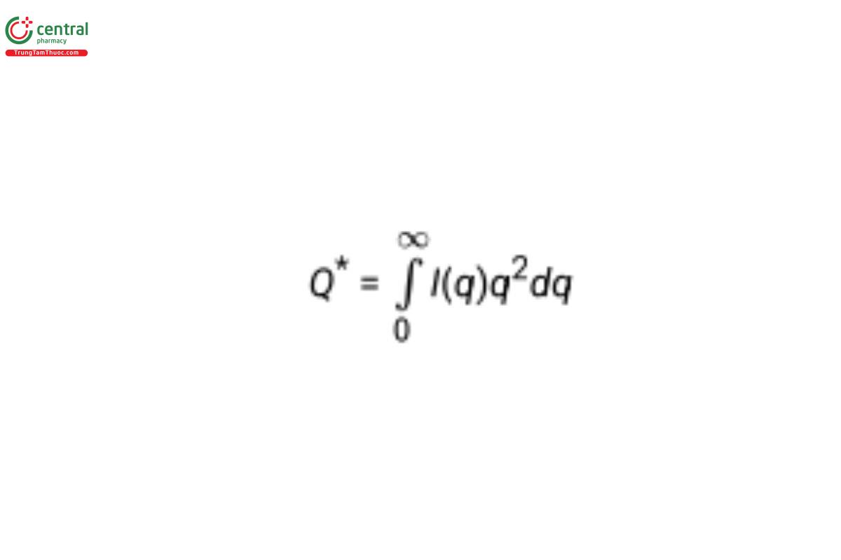
• The PDDF depicts the relative number of instances that two points in each scattering object are separated by a given distance, r. It is a function of distance only and is not a three-dimensional representation of the structure. The more symmetric the curve, the more rotationally symmetric the shape of the scattering object. Basic shapes like spheres, rods, and disks produce distinct distributions.
• Ab-initio methods:
○ Involve the iterative creation of complex-shape envelopes, for example, from assemblies of homogeneous spheres ordered on a lattice or using spherical harmonic functions, the computed scattering of which is then compared with the experimental I(q) data (14,15)
○ Are particularly useful for approximating the tertiary structure of biological molecules, but can also be applied to self-assembled soft matter systems like micelles
○ Do not take into account the chemical physics of the sample (e.g., bond lengths, bond angles, packing fractions, electrostatics)
○ Are computationally modest
• Simulation methods:
○ Involve the iterative manipulation of atomistic structures, for example, as derived from X-ray or high-resolution NMR crystal structures, by Boltzmann-weighted Monte Carlo/Molecular Dynamics methods, the computed scattering of which is then compared with the experimental I(q) data (16,17)
○ Are particularly useful for determining the tertiary structure of biological molecules
○ Take into account the chemical physics of the sample
○ Are computationally expensive, but can be used with coarse-graining methods
As SAS data analysis procedures become ever more sophisticated, so too does the degree of detail about the sample that they can return. However, one must never take this information in isolation; always look to cross-validate it with information derived from alternative techniques or the scientific literature. For example, model-fitting a large number of parameters without a priori information can result in “local” rather than “global” solutions. And PDDF, ab initio, and simulation methods work best when they can be constrained (e.g., to a known radius-of-gyration).
