ANALYTICAL METHODOLOGIES BASED ON SCATTERING PHENOMENA—GENERAL
If you find any inaccurate information, please let us know by providing your feedback here

Tóm tắt nội dung
This article is compiled based on the United States Pharmacopeia (USP) – 2025 Edition
Issued and maintained by the United States Pharmacopeial Convention (USP)
1 1. OVERVIEW: GENERAL CHAPTERS BASED ON SCATTERING PHENOMENA
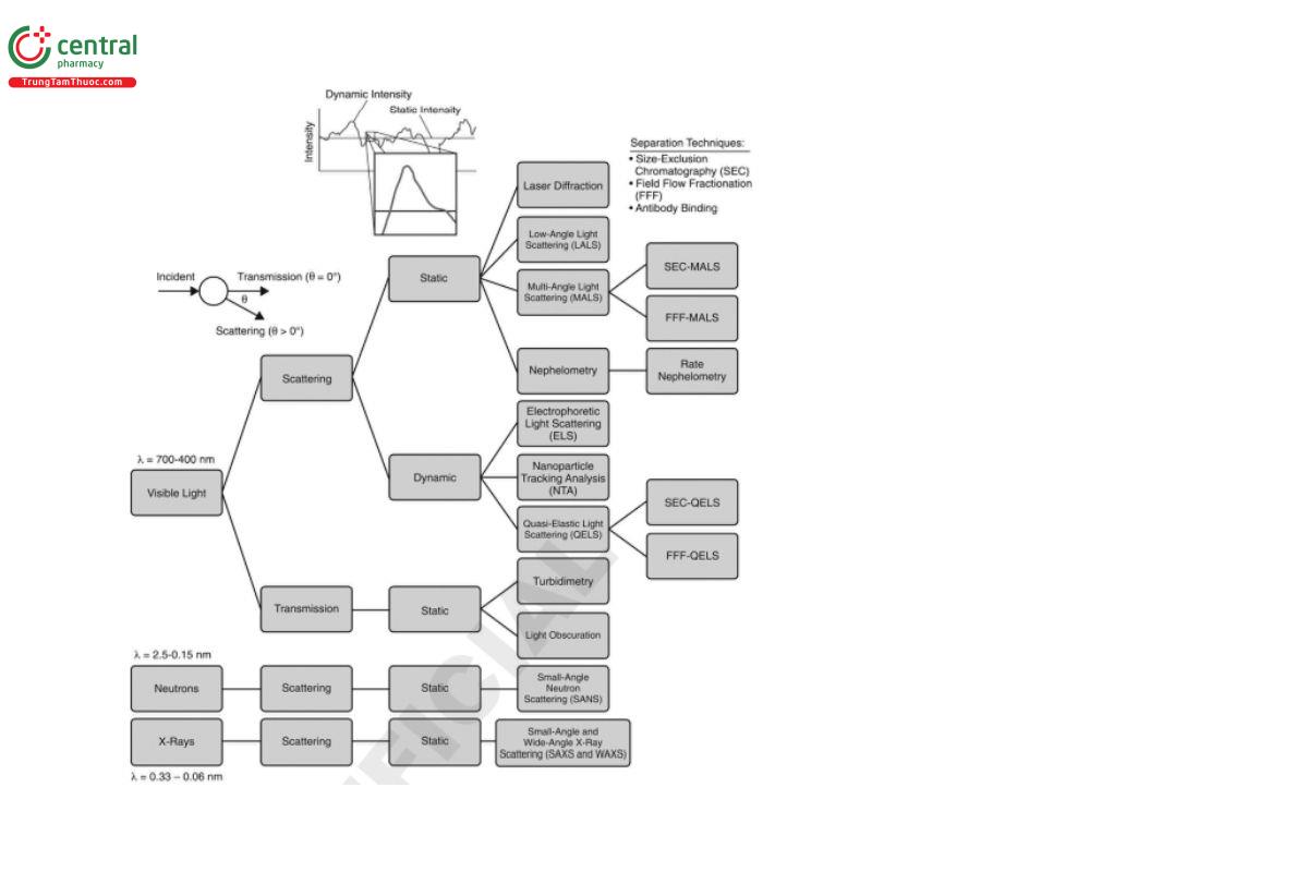
This chapter provides a general overview of the scientific principles and analytical procedures used in scattering techniques and their applications. Figure 1 shows a taxonomy (tree diagram) of the techniques that are covered in this chapter.
The first branch classifies the techniques according to the wavelength of the incident electromagnetic (EM) radiation:
visible light (700–400 nm)
X-rays (0.33–0.06 nm)
neutrons (2.5–0.15 nm)
The next branch classifies techniques into those based on the measured intensities (i.e., scattering), where the radiation exiting the sample is measured at an angle relative to the incident beam, or transmission, where this angle is equal to zero.
Scattering techniques can be further classified based on how the exiting radiation is quantified, in either a time-averaged (static) or time-dependent (dynamic) mode.
Finally, because scattering techniques are often coupled with separation techniques, such as chromatography or field flow fractionation, these are included as well.
Two of the most important parameters of the EM radiation–matter interaction are:
the wavelength of the incident EM radiation
(λ = λ₀ / m)
where λ₀ is the wavelength in vacuo and m is the refractive index of the medium
and
the size of the particle, often expressed as an equivalent spherical radius (r)
A dimensionless parameter
α = 2πr / λ
can be used to describe different scattering regimes.
For α << 1
the scattering is considered as being in the Rayleigh regime and the Rayleigh scattering theory applies.
For α ≈ 1
the scattering is considered as being in the Mie regime and the Mie scattering theory applies.
For α >> 1
geometric optics apply.
These theories are further addressed in the respective chapters where they are applied.
Table 1 lists all chapters whose fundamental physical principles are addressed in this overarching chapter. These chapters deal with elastic light scattering in heterogeneous systems and its applications in the pharmaceutical industry.
Table 1. List of 〈1430.X〉 General Chapters Family
| Chapter Number | Chapter Title | Measured Property | Primary Purpose |
|---|---|---|---|
| (1430) | Analytical Methodologies Based on Scattering Phenomena—General | Overarching chapter | General overview; N/A |
| (1430.1) | Analytical Methodologies Based on Scattering Phenomena—Static Light Scattering | Scattered light intensity as a function of detector’s angle | Molecular weight, size, shape; molecular interactions |
| (1430.2) | Analytical Methodologies Based on Scattering Phenomena—Light Diffraction Measurements of Particle Size | Diffracted light intensity at multiple angles | Particle size distributions in the approximate range of 0.01–3000 µm |
| (1430.3) | Analytical Methodologies Based on Scattering Phenomena—Dynamic Light Scattering | Fluctuations of the scattered light intensity | Average hydrodynamic diameter and polydispersity index |
| (1430.4) | Analytical Methodologies Based on Scattering Phenomena—Electrophoretic Light Scattering (Determination of Zeta Potential) | Doppler shift of scattered light frequency | Stability of suspensions and emulsions |
| (1430.5) | Analytical Methodologies Based on Scattering Phenomena—Small-Angle X-Ray Scattering and Small-Angle Neutron Scattering | Scattered intensity of a beam of X-rays or neutrons | Direct probing of the size, shape, ordering, and interactions of individual molecules, their assemblies in the approximate length scales from 0.1–2500 nm for SAXS and 0.2–1000+ nm for SANS. Also properties of condensed phases (e.g., porosity and crystallinity) can be determined. |
| (1430.6) ▲ (ERR 1-Oct-2021) | Analytical Methodologies Based on Scattering Phenomena—Particle Counting via Light Scattering | Light scattered from individual particles passing through a light beam | Quantitation of particles in liquids and gases from 0.1–2 µm |
| (1430.7) ▲ (ERR 1-Oct-2021) | Analytical Methodologies Based on Scattering Phenomena—Nephelometry and Turbidimetry | Direct or indirect measurement of the scattered light intensities | Suspended particles in liquid or gas samples; nephelometry for lower aggregate sizes and analyte concentrations; turbidimetry for higher aggregate sizes and analyte concentrations |
Because these methods are based on the same underlying physics, the general principles are given only once in this overarching chapter.
The relationships between these methods are shown in Figure 1.
2 2. INTRODUCTION
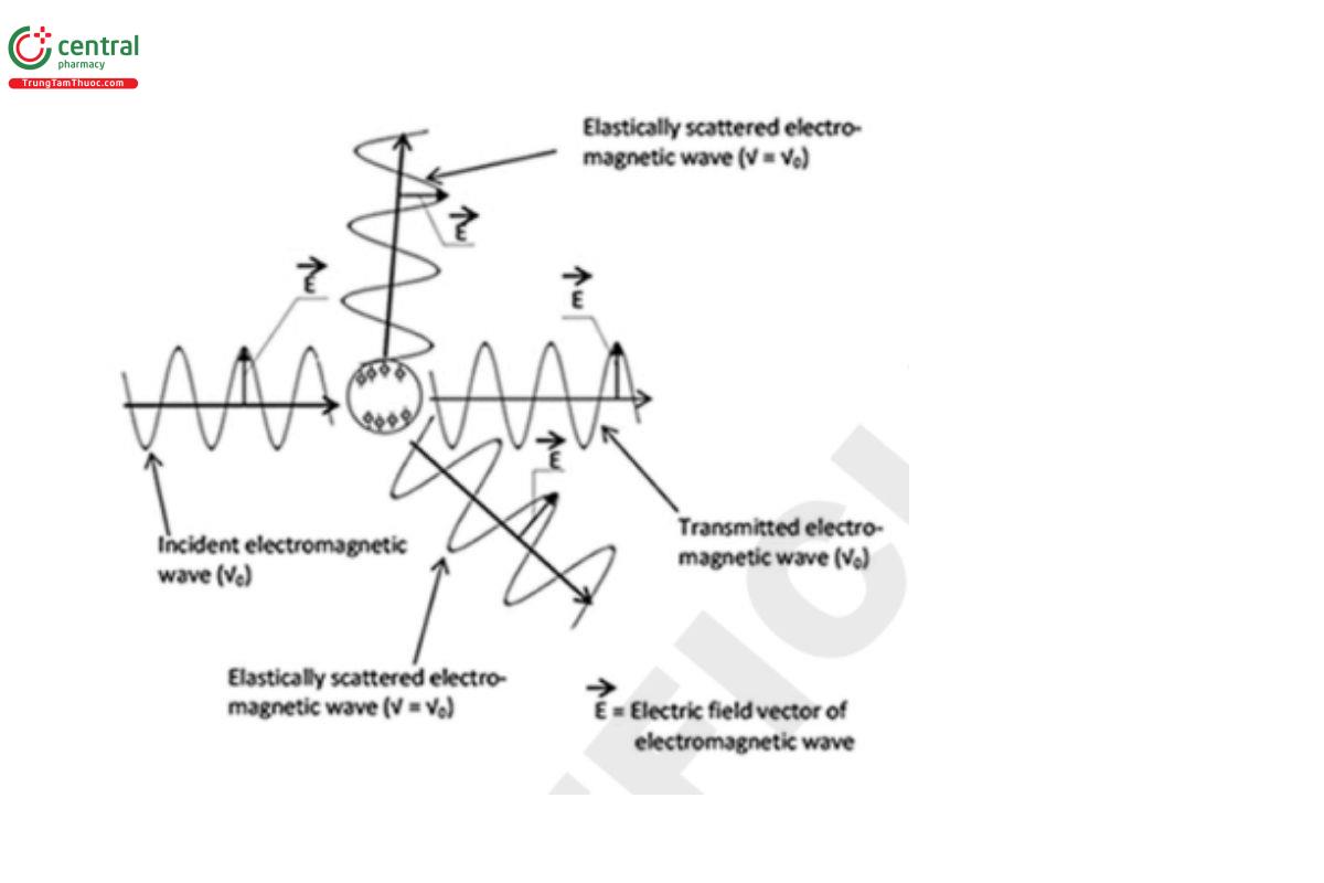
When an EM wave strikes/interacts with a small object (a particle or a molecule) and thereby changes its direction, the phenomenon is called scattering.
If the scattered EM radiation has exactly the same energy (wavelength) as the incident one, it is called elastic scattering.
When the energy (wavelength) of the scattered EM radiation is different from that of the incident EM radiation, the scattering process is termed “inelastic”.
Inelastic scattering is exploited, as an example, by Raman spectroscopy (refer to Raman Spectroscopy—Theory and Practice 〈1858〉).
Scattered radiation may be detected and measured either:
directly: as a function of the angle between the incident beam direction and the detector
or
indirectly: when the actual measurement is that of the transmitted light.
The latter is the case for both turbidity and light obscuration methods (see the following chapters on turbidity and light obscuration):
Nephelometry, Turbidimetry, and Visual Comparison 〈855〉
Subvisible Particulate Matter in Therapeutic Protein Injections 〈787〉
Particulate Matter in Injections 〈788〉
Methods for the Determination of Subvisible Particulate Matter 〈1788〉
Both methodologies exploit time averaged signals.
In static light scattering (SLS), the inevitable short-term temporal fluctuations in scattering intensity due to Brownian motion are averaged over a range of times from tens to hundreds of milliseconds.
SLS therefore measures the “time average” intensity of scattered light from particles in a (suitably prepared) sample.
Depending on the specific technique, SLS provides information about:
molecular weight
particle size
particle shape
molecular interactions
(see Analytical Methodologies Based on Scattering Phenomena—Static Light Scattering 〈1430.1〉).
Light scattered in the near-forward direction by particles is analogous to diffraction of light through an aperture.
This is exploited by (laser) diffraction techniques, which are optimized to afford the derivation of a full size distribution, with moderate to high resolution, rather than a single characteristic size as in low-angle light scattering (LALS)/multi-angle light scattering (MALS).
Small-angle X-ray scattering (SAXS) and small-angle neutron scattering (SANS) are also static techniques in that they make use of time averaged signals.
These differ from LALS (and MALS) in that they are based on scattering of X-rays (SAXS) or neutrons (SANS) rather than visible light.
Like SLS, these techniques also measure size, shape, and interactions but on much shorter length scales, typically ranging from around 1 nm to several hundred nanometers.
Very/ultra small-angle (VSAXS/VSANS, USAXS/USANS) and wide-angle (WAXS/WANS) analogues extend these length scales to the micrometer and sub-nanometer regimes, respectively.
These applications are discussed in Analytical Methodologies Based on Scattering Phenomena—Small-Angle X-Ray Scattering and Small-Angle Neutron Scattering 〈1430.5〉.
Dynamic light scattering (DLS), which is addressed in Particle Size Analysis by Dynamic Light Scattering 〈430〉 and Analytical Methodologies Based on Scattering Phenomena—Dynamic Light Scattering 〈1430.3〉, differs from SLS in that DLS measures the fluctuation of the scattered light intensity over very short time intervals (e.g., approximately 200, 400 ns).
Electrophoretic light scattering (determination of zeta potential), which is addressed in more detail in Determination of Zeta Potential by Electrophoretic Light Scattering 〈432〉 and Analytical Methodologies Based on Scattering Phenomena—Electrophoretic Light Scattering (Determination of Zeta Potential) 〈1430.4〉, measures the Doppler shift of the frequency of scattered light as the result of particle movements from the cumulative effect of electrophoresis and electroosmosis.
3 3. THEORY (GENERAL PRINCIPLES OF SCATTERING)
Light/EM scattering is the result of a complex interaction between incident light/EM waves and matter.
An EM wave that is redirected, i.e. changes direction, when it encounters obstacles such as a molecule or molecular aggregates, or particles, is said to have been scattered.
As the EM radiation, such as light or X-rays, interacts with a discrete particle, the electron orbits within the particle’s constituent atoms or molecules are perturbed periodically with the same frequency (ν₀) as the electric field of the incident wave.
The oscillation or perturbation of the electron cloud results in a periodic separation of charge within the molecule, which is called an induced dipole moment.
The oscillating induced dipole moment manifests itself as a source of EM radiation. Neutrons, on the other hand, are always scattered by a very short-range nuclear interaction with the nuclei in the atoms.
The (time averaged) intensity (I) of the light beam as it interacts with matter along its path (i.e., when the incident light is detected at an angle of zero) decreases exponentially with the thickness, x, of the layer of material as follows in Equation 1: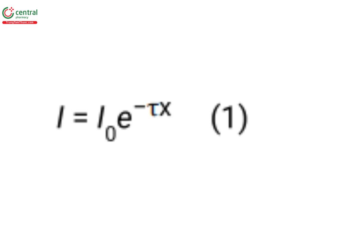
where τ is the turbidity and x is the distance that the incident light travels through the sample.
This equation is the basis for turbidimetry and nephelometry (see 〈855〉).
In SLS, the theoretical description of the relationship between the (time averaged) intensities of incident and scattered light, although quite complex, originates from the following simple relationship (Equation 2):
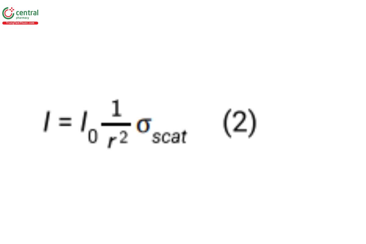
The scattering coefficient, σ_scat, and with it the intensity of the scattered light depend on factors determined by the interaction of the incident light with the material/particles itself as well as those stemming from the equipment used for generating and detecting the signal (e.g., r, the distance of the detector from the sample; I₀, the intensity of the incident light; and Θ, the angle of observation).
On the other hand, when studying the fluctuations in scattered intensity (DLS), the way to extract useful, quantitative information is by calculating the so-called “autocorrelation function”, denoted g₂(τ) based on the measured intensities (Equation 3):
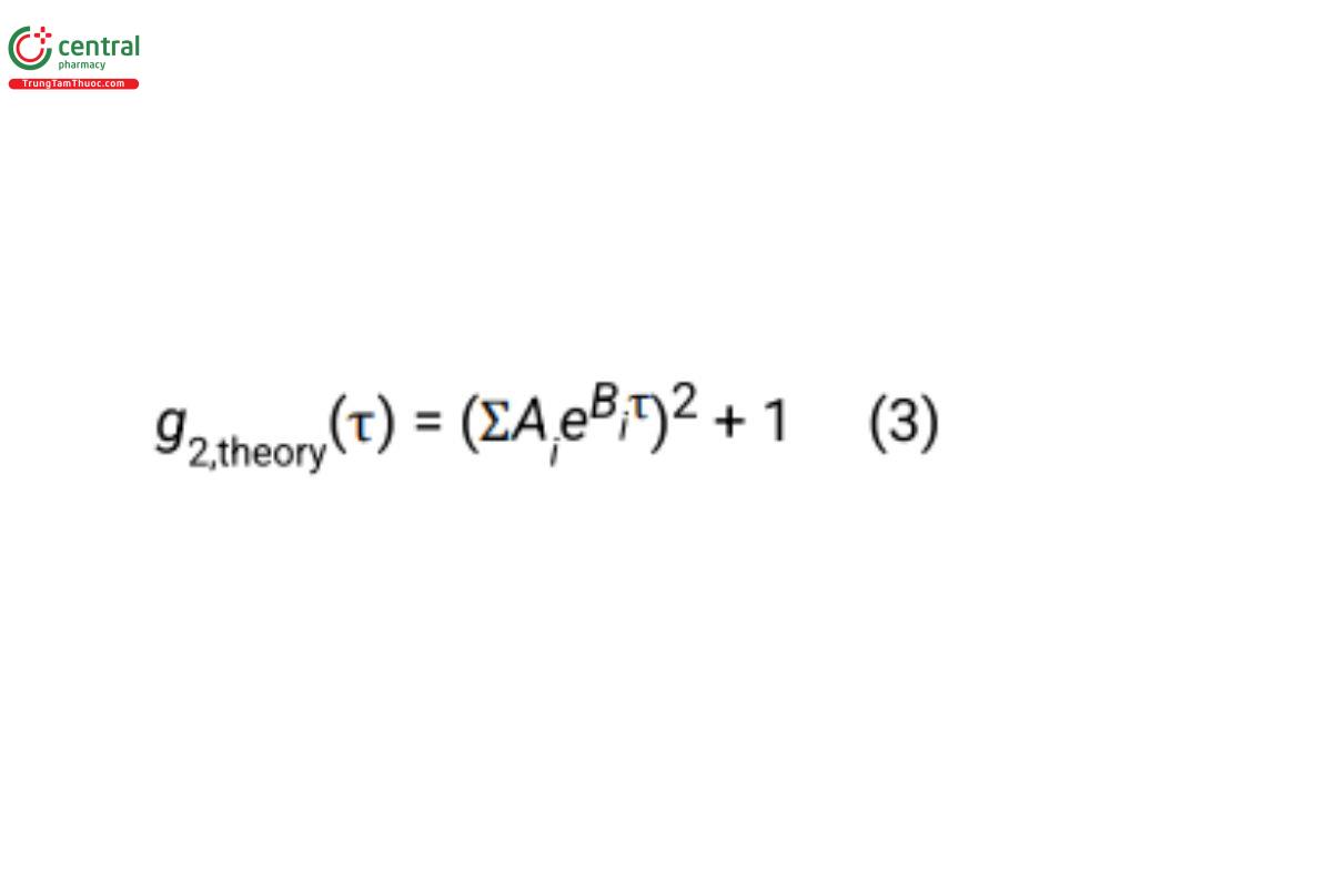
where in this case, τ denotes a correlation time (not to be confused with the τ in Equation 1 above), and the use of the index, i, accounts for different particle types (e.g., different sizes) present.
A computer program is used to find the parameters A, B (= A₁, B₁, A₂, B₂, …) that produce the best agreement between the measured and theoretical autocorrelation function.
Depending on the methodology, the equations above are transformed to obtain a measure that relates the measured intensities, I and I₀, respectively, and the autocorrelation function g₂(τ) to the material itself, independent of equipment characteristics.
These are further discussed in the specific chapters in the USP–NF dedicated to the corresponding techniques (see Table 1).
