ANALYTICAL METHODOLOGIES BASED ON SCATTERING PHENOMENA - STATIC LIGHT SCATTERING
If you find any inaccurate information, please let us know by providing your feedback here

Tóm tắt nội dung
This article is compiled based on the United States Pharmacopeia (USP) – 2025 Edition
Issued and maintained by the United States Pharmacopeial Convention (USP)
DOWNLOAD PDF HERE
1 INTRODUCTION
The phenomena observed when photons [i.e., an electromagnetic (EM) wave] strike or interact with a small object (a particle or a molecule) and thereby change direction is called light scattering (LS).
In static light scattering (SLS), the inevitable short-term temporal fluctuations in scattering intensity due to Brownian motion are averaged over a range of time scales from several hundredths to several tenths of a second. SLS measures the time average intensity of scattered light from particles in a suitably prepared sample; the detector signal is, therefore, time independent or “static”.
In SLS, the scattered light is detected and measured as a function of the angle between the detector and the incident beam direction. Light scattering can be either at a single fixed angle, as in low-angle light scattering (LALS) or right-angle light scattering (RALS); or over a range of angles, as in multi-angle light scattering (MALS).
SLS provides information about molecular weight, particle size, particle shape, and molecular interactions.
This chapter provides guidance and procedures for LALS and MALS. These SLS methodologies are based on the Rayleigh approximation of classical Mie scattering theory. In these scattering methods, the particles are assumed to be present in solution (or gas) and free to move; thus, the particles are inherently in an unordered state. Other scattering phenomena such as reflection, refraction, and diffraction require the scattering particles to be highly ordered and are out of the scope of this text.
2 THEORY
SLS techniques are based on measurement(s) of the scattered light intensity (I ) itself, as opposed to indirect measurements (e.g., IS inferring the scattered intensity from the attenuation of transmitted light).
In order to obtain a measure that relates the material itself to the scattering intensity, independent of equipment characteristics, one defines the Rayleigh ratio, R(Θ), for the sample under investigation (Equation 1):
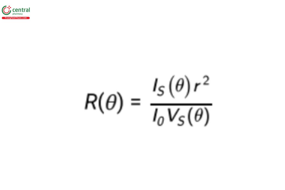
R(Θ) is defined as the scattered intensity per unit solid angle, scattering volume (VS), and incident intensity (I0) that is in excess of that scattered by solvent alone, and r is the distance of the scattering volume from the detector.
Figure 1 shows that the scattering of light on the particle changes the wave vector from kincident to ~kscatter. For sufficiently small particles, only the direction, but not the wavelength, changes as a result of the collision. Hence, the length of the wave vector k remains unchanged.
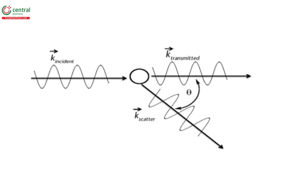
As the EM wave interacts with the electron orbits of the constituent molecules, the orbits are perturbed periodically at the same frequency as the electric field of the EM wave. The oscillations of bound and free charges in turn generate EM waves inside and outside of the particle.
Although Maxwell’s equations for an EM light wave interacting with a sphere completely describe these interactions, proper boundary conditions for electric and magnetic fields are needed to find the exact solutions for these equations, along with the values of the quantities of interest. Moreover, such solutions are difficult to find.
One of the rare exact solutions for the scattering of a plane wave by a uniform sphere is obtained from the Mie theory of scattering (1). Mie theory has no size limitations; it converges to the limit of geometric optics for large particles. Mie theory, therefore, may be used to describe most spherical particle scattering systems. However, difficulties in finding exact solutions for the wave equations have led to the development of approximate methods of solving the scattering problem. One class of these approximations, known as Rayleigh scattering theory, describes light scattering by particles that are small compared to the wavelength of the light (2,3). Due to the complexity of the Mie scattering solution, the Rayleigh scattering theory is generally preferred, if applicable.
When the scattering particles are much smaller than the wavelength of the light (approximately 1/20 of the wavelength or less), they are considered to be at the Rayleigh scattering regime. The EM field acting on the particle in the Rayleigh scattering regime is effectively homogenous. This is a very important approximation for biomedical optics because many of the structures from which cell organelles are built (e.g., the tubules of the endoplasmic reticulum, cisternae of the Golgi apparatus) fall into this category.
Therefore, the time for penetration of the electric field is much shorter than the period of oscillation of the EM wave. The particle behaves like a dipole and therefore radiates (scatters) light isotropically, i.e., at an equal intensity in all directions relative to the direction of the incident light. With larger particles and/or shorter wavelengths, the scattered light begins to exhibit additional interference effects from other atoms within the molecule.
In addition, the scattered light has the same wavelength as the incoming light, a process referred to as elastic scattering. Moreover, the intensity of the scattered light is independent of the particle size.
At the Rayleigh limit, the Rayleigh ratio is transformed to Equation 2:
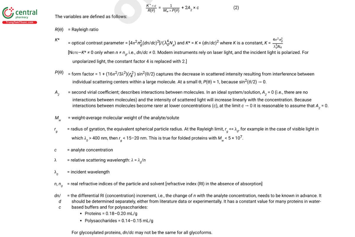
NA = Avogadro constant
3 APPLICATIONS
3.1 Low-Angle Light Scattering Determination of Molecular Weight
Depending on the experimental conditions, it is possible to further simplify Equation 2, thereby making it amenable to practical applications. In particular, at small scattering angles, Θ → 0, P(Θ) → 1. Therefore, at small angles, scattering is independent of Θ. This observation forms the basis of LALS. Note that measurements at Θ = 0 are impractical because the incident (laser) light would interfere with the measurement.
3.1.1 MEASUREMENTS AT LOW CONCENTRATION
Further, at the limit of low concentrations, the term A2 × c approaches 0. Equation 2 then simplifies to Equation 3, as shown below:
RLS(θ) = KLS × c × MW × (dn/dc)2 (3)
A prerequisite prior to applying the above equation is an accurate determination of the value of dn/dc, which is dependent on both the solvent and the sample/analyte. The value of dn/dc can be determined experimentally by measuring the RI of the sample in a known solvent at various concentrations. The slope of the regression line of n versus c is then dn/dc.
For example, for a protein or complex that contains no carbohydrate, dn/dc is constant (often ≈ 0.185 mL/g) and nearly independent of the Amino acid composition of the protein. However, it is advised to measure the actual dn/dc for each material in order to obtain an accurate result.
3.1.2 MEASUREMENTS AT MULTIPLE CONCENTRATIONS
When data are available at several concentrations, the second virial coefficient, A2, may be determined (see Equation 2).
To determine the molecular weight, Mw, from measurements at different concentrations and at low angles [at which P(Θ) ≈ 1], use Equation 2:
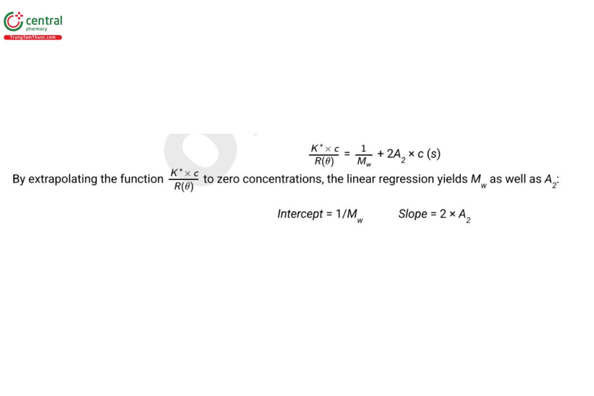
However, the molecular weight obtained by this approach is very sensitive to the molecular polydispersity of the sample as well as interference by impurities.
3.1.3 COMBINATION WITH OTHER DETECTION TECHNIQUES
Determination of Mw by LALS stipulates that dn/dc is known. To this end, the RI increment, dn/dc, has to be measured for several different concentrations to generate a plot of dn/dc versus c, the y-intercept of which is dn/dc. Alternatively, when dn/dc is constant, the slope of the regression line of n versus c is dn/dc. Determination of dn/dc is facilitated by the coupling of LALS with an RI detector, and Equation 4 is used for the RI signal, as shown below:
RRI(θ) = KRIcMw(dn/dc) (4)
Combining Equation 3 and Equation 4 leads to Equation 5, as shown below:
Mw = K′(LS)/(RI) (5)
where K′ = KRI/[KLS(dn/dc)] is the instrument calibration constant. The molecular weight Mw is then derived from the ratio of the LS versus the RI signal. This assumes that dn/dc is constant.
When dn/dc is no longer constant, for example in the case of carbohydrate-containing proteins, an additional detector is needed. For samples detectable by UV, a wavelength is chosen at which ε for the carbohydrate but not the protein part is = 0. Then the ε in Equation 6 below is effectively that of the protein:
UV = KUVCε (6)
The value of the specific refractive increment, dn/dc, can then be assumed to be proportional to (RI)A/(UV). The outputs of the three detectors, designated LS, RI, and UV, respectively, are related to the molar mass of a sample according to Equation 7, as shown below:
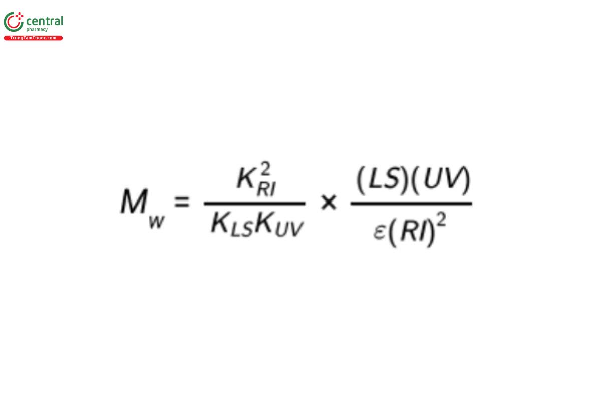
ε is a material but not an equipment constant and usually must be determined separately.
3.2 Multi-Angle Light Scattering
In MALS, measurements are made at multiple angles (at least three). To obtain the values of the three unknowns on the right-hand side of Equation 2 (Mw, A2, and the mean square radius, rg2 ), measurements of R(Θ) at three different angles are needed in order to obtain three independent expressions of Equation 2. The number of angles at which measurements are made (i.e., the quantity of data collected) determines the precision (reproducibility) as well as the accuracy of the measurement.
By measuring the angular dependence of the signal, it is possible to calculate the molecular size (rg) from the initial slope (at small angles) of the angular dependence in Equation 8, as shown below:
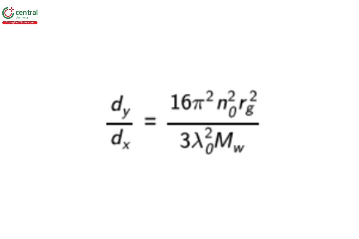
where n0 is the RI of the solvent, rg is the root mean square radius (radius of gyration, molecular size), λ0 is the vacuum wavelength of the laser, and Mw is the molecular weight.
In addition, measuring the signal over multiple angles provides information on the three-dimensional shape of the analyte, either by using non-linear regression analysis or graphically by using Zimm plots (4).
3.3 Combination of Light Scattering with Size-Fractionation Techniques
A more robust approach to molecular weight determination is based on pre-fractionation of poly-disperse protein mixtures or analytes into “slices” of uniform molecular weight. The coupling of fractionation and detection techniques affords more information than either method can provide on its own.
Size-fractionation techniques include size exclusion chromatography (SEC), field-flow fractionation (FFF) techniques, and other separation modes. By applying light scattering in combination with another concentration detector such as RI or UV, a more complete description of the molecular weight distribution can be realized.
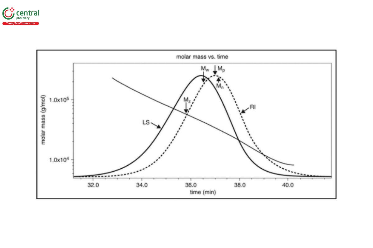
Figure 2 shows an example of this for a sample of Dextran with a known molecular weight of approximately 40 kDa. The diagonal line shows the molecular weight across the SEC curve, and the entire distribution can be used to calculate molecular weight moments; the most obvious one is Mp, which is the molecular weight at the peak of the distribution. In addition, three other parameters can be calculated:
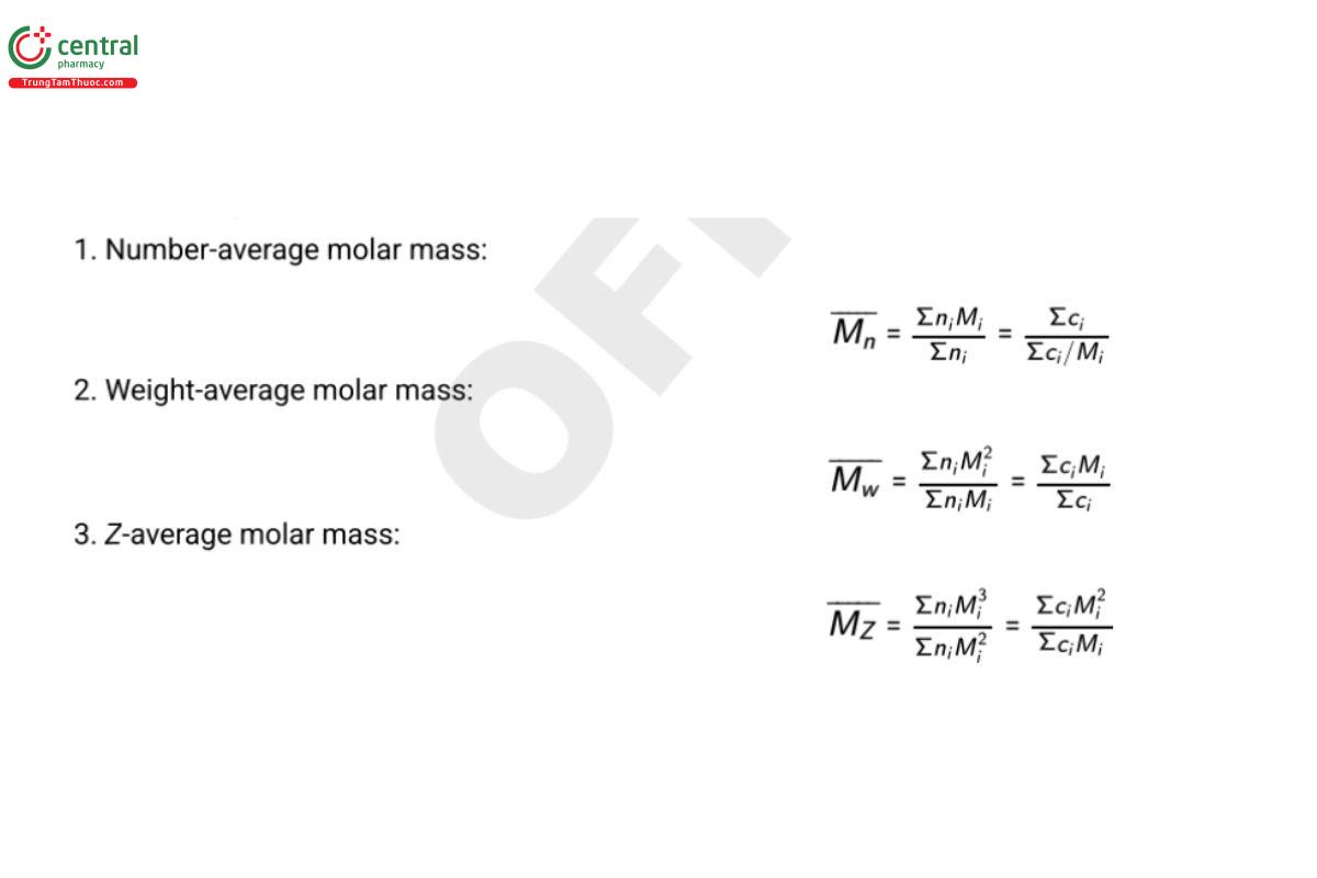
The value of ni is the number of molecules with molar mass Mi, and ci is the weight concentration of molecules with molar mass Mi (as determined by the RI detector).
In the case of 40 kDa Dextran, the measured parameters are shown in Table 1, along with a calculation of the polydispersity (Ip = Mw/Mn).
Table 1. Measured Molar Mass Parameters for 40 kDa Dextran
| Parameter | Value |
| Mn | 29,420 |
| Mp | 34,650 |
| Mw | 40,760 |
| Mz | 55,960 |
| Ip (= Mw/Mn) | 1385 |
Figure 2. Molecular weight distribution for 40 kDa Dextran.
4 INSTRUMENTATION
Modern light scattering spectrometers use laser light because of the following advantages that lasers offer over conventional light sources:
- Reliability
- Beam collimation
- Single wavelength (scattering depends on the wavelength of the scattered light)
- Equipment durability and compactness
Figure 3 shows a typical setup for the measurement of SLS. A monochromatic light source (i.e., a light source emitting light of only one wavelength; usually a laser) shines light on the sample. The intensity or the power of the scattered light is being measured at a known scattering angle Θ by a detector.
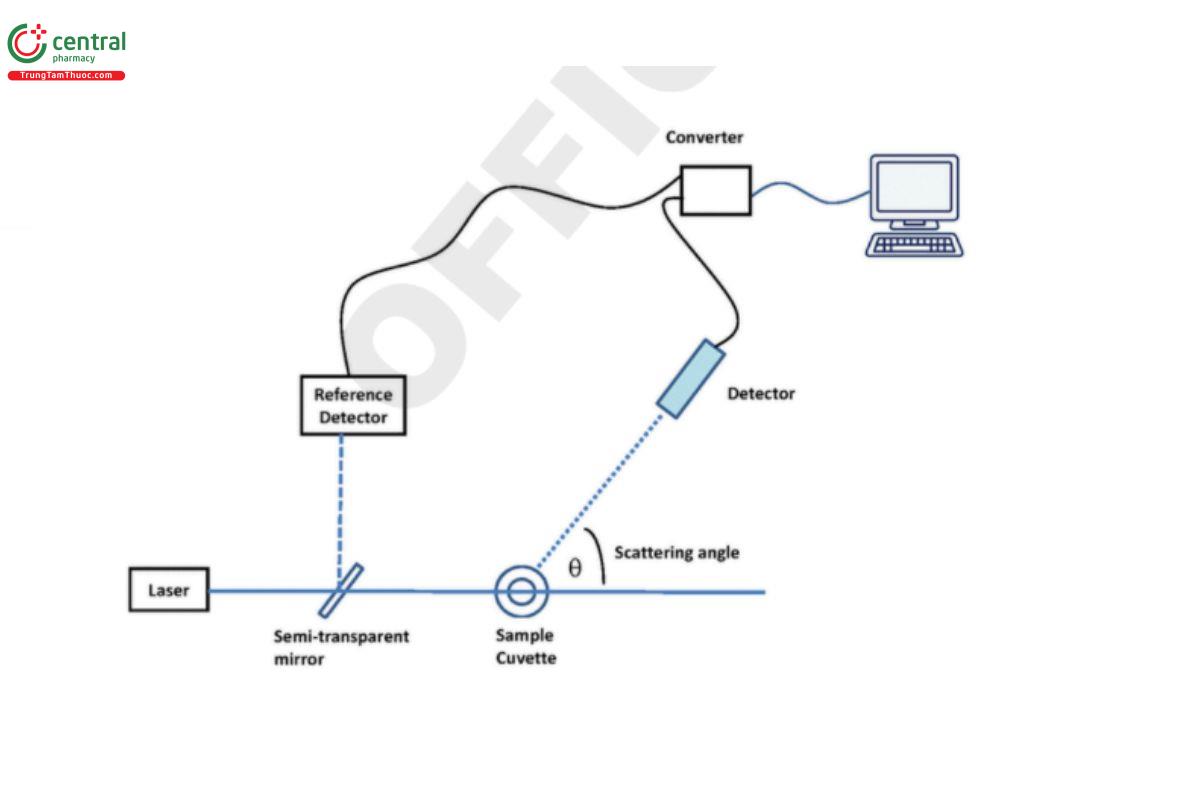
Figure 3. A typical setup of a static light-scattering instrument.
Historically, the measurements at different angles were made using a scanning photometer (single detector, variable angle). More recently, photometers containing a fixed array of 3–18 detectors have come into use.
5 LOW-ANGLE LIGHT SCATTERING VERSUS MULTI-ANGLE LIGHT SCATTERING
A major advantage of LALS is the exact measurement of high molecular weights (>10 million g/mol) without the principle-related errors that often occur with extrapolations, which are necessary for measurements at higher angles (but not with the use of many angles).
The major drawbacks of LALS when compared to MALS are as follows:
- Higher noise: Low angles are always noisier than high angles. Although using in-line filter(s) removes the scattering effects of debris from the low-angle data, it also removes much of the signal. Further, the measurement precision is roughly proportional to the square root of the number of detectors.
- Less information: Multi-angle data are needed to solve the Rayleigh equations.
- Inability to obtain information on molecular shape (see 3.2 Multi-Angle Light Scattering).
LALS techniques and systems may be preferred for their simplicity and have been optimized to deal with their inherently lower information content (e.g., linearization strategies of multi-concentration data such as Zimm plots). Low-angle systems will be much cheaper and less dependent than the more complex equipment and (proprietary) fitting algorithms used in multi-angle systems. Finally, with the use of additional coupled simple detector systems such as RI and UV, the determination of molecular weight using LALS is a feasible, robust option.
A combination of the simplicity of LALS with the improved signal-to-noise ratio of higher scattering angles, offered by modern detectors, is achieved when performing measurements at Θ = 90°, the angle with the highest signal-to-noise ratio. Also, except for proteins of high molecular weight, there will be no significant angular dependence of the scattering with this configuration. However, for high molecular weight proteins, the light scattering signal has to be corrected with a viscosity detector, which requires making additional theoretical assumptions that are difficult to verify for routine applications.
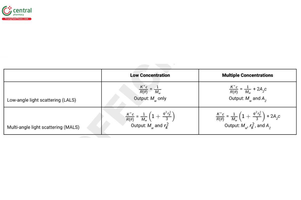
6 PRACTICAL CONSIDERATIONS
Many SLS experiments, particularly those aimed at elucidating properties of proteins and other polymers in solution, will fall into the Rayleigh–Gans–Debye (RGD) scattering regime. Table 2 summarizes the governing equations for four typical experimental situations: 1) low- angle scattering at a low concentration, which provides information on the molecular weight of the sample; 2) low-angle scattering at multiple concentrations, which provides information on molecular weight and solution non-ideality; 3) multi-angle scattering at a low concentration, which provides information on molecular weight and molecular size; and 4) multi-angle scattering at multiple concentrations, which provides information on molecular weight, molecular size, and solution non-ideality.
Table 2. Most Common Governing Equations
Additional considerations:
- To obtain a reliable estimate for the excess Rayleigh ratio, one must use a calibration standard to obtain an “absolute” scattered intensity. Pure organic solvents (e.g., toluene) can be used for this purpose. It is important to note that the Rayleigh ratio of the solvent is a function of wavelength of the incident light. Alternatively, one can calibrate the system using a standard of known molecular weight (e.g., bovine serum Albumin).
- For the above RGD equations to hold, samples must not absorb light in the wavelength range of the incident beam. Because laser light in the visible range is most common, samples should be colorless. If the samples are colored, more advanced data analysis techniques are required. Otherwise, the results will be unreliable.
- Likewise, cuvettes in the instrument systems with removable cuvette should not absorb light in the wavelength range of the incident beam. Care should be taken to ensure that the cuvette is free from smudges, scratches, or any other optical defect that could interfere with the measurement.
- Scattered intensity depends on the molecular size. Very small levels of large particles can dominate the signal and compromise the measurement. Samples should be appropriately prepared to minimize contamination from environmental or other sources. Sample preparation may include filtration, centrifugation, or other appropriate separation techniques. Care should be taken to ensure that the method of sample preparation itself does not introduce experimental artifacts (e.g., the analyte of interest adsorbing to a filter membrane). It is good practice to examine samples by dynamic light scattering to verify the absence of large contaminating species prior to conducting SLS measurements.
7 ADDITIONAL SOURCES OF INFORMATION
Hahn DW. Light scattering theory. University of Florida; 2009. http://plaza.ufledu/dwhahn/Rayleigh%20and%20Mie%20Light%20Scattering.pdf.
Kaye W, Havlik AJ, McDaniel JB. Light scattering measurements on liquids at small angles. J Polym Sci C. 1971;9(9):695–699.
Øgendal L. Light scattering: a brief introduction. University of Copenhagen; 2016. http://www.nbi.dk/~ogendal/personal/lho/LS_brief_intro.pdf.
Takagi T. Application of low-angle laser light scattering detection in the field of biochemistry: review of recent progress. J Chromatogr A. 1990;506:409–416.
Wen J, Arakawa T, Philo JS. Size-exclusion chromatography with on-line light-scattering, absorbance, and refractive index detectors for studying proteins and their interactions. Anal Biochem. 1996;240(2):155–166.
8 REFERENCES
- Mie G. Contributions to the optics of turbid media, particularly of colloidal metal solutions. Ann Phys. 1908;25(3):377–445.
- Strutt JW. On the scattering of light by small particles. Philos Mag. 1871;41(275):447–454.
- Strutt JW. On the electromagnetic theory of light. Philos Mag. 1881;12(73):81–101.
- Wyatt PJ. Light scattering and the absolute characterization of macromolecules. Anal Chim Acta. 1993;272(1):1–40. (USP 1-Dec-2019)
