Analytical Data—Interpretation and Treatment

This article is compiled based on the United States Pharmacopeia (USP) – 2025 Edition

Issued and maintained by the United States Pharmacopeial Convention (USP)

DOWNLOAD PDF HERE

1 INTRODUCTION

This chapter provides information regarding acceptable practices for the use of analytical procedures to make decisions about pharmaceutical processes and products. Basic statistical approaches for decision making are described, and the comparison of analytical procedures is discussed in some detail.

[Note—It should not be inferred that the analysis tools mentioned in this chapter form an exhaustive list. Other, equally valid, statistical methods may be used at the discretion of the manufacturer and other users of this chapter.]

Assurance of the quality of pharmaceuticals is accomplished by combining a number of practices, including rigorous process and formulation design, development, validation, and execution of a robust control strategy. Each of these is dependent on reliable analytical procedures. In the development process, analytical procedures are utilized to ensure that the manufactured products are thoroughly characterized and to optimize the commercial manufacturing process. Final-product testing provides assurance that a product is consistently safe, efficacious, and in compliance with its specifications. Sound statistical approaches can be included in the commercial control strategy to further ensure that quality is preserved throughout the product life cycle.

While not meant to be a complete account of statistical methodology, this chapter will rely upon some fundamental statistical paradigms. Key among these are population parameters, statistical design and sampling, and parameter uncertainty. Population parameters are the true but unknown values of a scientific characteristic of interest. While unknown, these can be estimated using statistical design and sampling. Statistical design is used to fully represent the population of interest and to manage the uncertainty of a result, while the random acquisition of test samples as well as their introduction into the measurement process helps to mitigate bias. Lastly uncertainty should be acknowledged between the true population parameter and the estimation process. Uncertainty can be expressed as either a probabilistic margin between the true and estimated value of a population parameter (e.g., a 95% confidence interval) or as the certainty that the population parameter is compliant with some expectation or acceptance criterion (predictive probability).

This chapter provides direction for scientifically acceptable administration of pharmaceutical studies using analytical data. Focus is on investigational studies where analytical data are generated from carefully planned and executed experiments, as well as confirmatory studies which are strictly regulated with limited flexibility in design and evaluation. This is in contrast to exploratory studies where historical data are utilized to identify trends or effects which are subject to further investigation. The quality of decisions made from either investigational or confirmatory studies is enhanced through adherence to the scientific method, and to the application of sound statistical principles. The steps of the scientific method can be summarized as follows.

Study objective. A pharmaceutical study can be as simple as testing and releasing a batch of commercial material or as complex as a comparison of analytical procedures. The same considerations apply to the simple study as they do to the complex study. Each study is associated with a population parameter which is used to address the study objective. For release, the parameter might be the batch mean. For the analytical procedure comparison study, the parameter might be the difference in means produced by the analytical procedures. In each case an appropriate acceptance criterion on the population parameter is used to make a decision from the study.

Study design. The study should be designed with a structure and replication strategy which ensures representative consideration of the study objective, and which manages the risks associated with making an incorrect decision. Representative consideration of the study objective entails inclusion of samples and conditions which span the population being studied. Thus in release of a manufactured lot, samples across the range of manufacture might be included, while in a procedure comparison, each type and level of test sample might be considered. Similar consideration should be given to sample testing, where appropriate factors should be included in the procedure. The design should also acknowledge the study risks. The statistical basis for managing study risk is the reduction of the uncertainty in the estimation of the population parameter.

Study conduct. Once the study has been designed, samples are collected and data are generated using the analytical procedure. Effective use of randomization should be considered to minimize the impact of systematic variability or bias. Care should be taken during data collection to properly control the analytical procedure and to ensure accurate transcription and preservation of information. An adequate number of significant digits or decimal places should be saved and used throughout the calculations. Deviations from the study plan should be captured and assessed for their potential to impact study decisions.

Study analysis and decision. Prior to the nal analysis, the data should be explored for data transformation and potential outliers. The analysis of the data should proceed according to the statistical methods considered during the study design. The analysis of the data and the reporting of study results should include proper consideration of uncertainty. Where appropriate, interval estimates should be used to communicate the robustness of the results (viz., the width of the interval) as well as facilitate communication of the study decision. A decision can be made when the objective of the study has been preformulated to make such a decision (e.g., as in an investigational or confirmatory study). The study may otherwise have been performed to estimate or describe some characteristic of a population. Caution should be taken in making decisions from post-hoc analyses of the data. This is called “data snooping” and can lead to inappropriate decisions.

This chapter has been written for the laboratory scientist and the statistician alike. The laboratory scientist is primarily skilled in the analytical procedures and the uses made of those procedures and should be aware of the value of statistical design and analysis in their practices. The statistician is primarily skilled in the design of empirical studies and the analysis which will return reliable decisions and should appreciate the science and constraints within the laboratories. While variously knowledgeable in their understanding across specialties, both disciplines should value the essential components that comprise uses of analytical data.

More detailed discussion related to the steps of the scientific method will be given in 4. Study Considerations and will be illustrated with an example in 5. Comparison of Analytical Procedures. Prior to this, there will be a section to review 2. Prerequisite Laboratory Practices and Principles and a section to describe and illustrate 3. Basic Statistical Principles and Uncertainty. A series of appendices is provided to illustrate topics related to the generation and use of analytical data. Control charts, equivalence and noninferiority testing, the principle of uncertainty, and Bayesian statistics are briefly discussed. The framework within which the results from a compendial test are interpreted is clearly outlined in General Notices, 7. Test Results. Selected references that might be helpful in obtaining additional information on the statistical tools discussed in this chapter are listed in References at the end of the chapter. USP does not endorse these citations, and they do not represent an exhaustive list. Further information about many of the methods cited in this chapter may also be found in most statistical textbooks.

2 PREREQUISITE LABORATORY PRACTICES AND PRINCIPLES

The sound application of statistical principles to analytical data requires the assumption that such data have been collected in a traceable (i.e., documented) and unbiased manner. To ensure this, the following practices are beneficial.

2.1 Sound Record Keeping

Laboratory records are maintained with sufficient detail, so that other equally qualified analysts can reconstruct the experimental conditions and review the results obtained. When collecting data, the data should be obtained with more decimal places than the specification or study acceptance criterion requires. Rounding of results from uses of analytical data should occur only after nal calculations are completed as per the General Notices. Study protocols and data analyses should be adequately documented so that a reviewer can understand the bases of the study design and the pathway to study decisions.

2.2 Procedure Validation

Analytical procedures used to release and monitor stability of clinical and commercial materials are appropriately validated as specied in Validation of Compendial Procedures 〈1225〉 or vefiried as noted in Verication of Compendial Procedures 〈1226〉. Further guidance is given in Statistical Tools for Procedure Validation 〈1210〉 and Biological Assay Validation 〈1033〉. Analytical procedures published in the USP–NF should be validated and meet the current good manufacturing practices (GMP) regulatory requirement for validation as established in the United States Code of Federal Regulations. When an analytical procedure is used in a non-GMP study, it’s good practice to ensure that the analytical procedure is adequately t for use to support the study objective.

2.3 Analytical Procedure and Sample Performance Verification

Verifying an acceptable level of performance for an analytical procedure in routine or continuous use is a valuable practice. This may be accomplished by analyzing a control sample at appropriate intervals or locations, or using other means, such as determining and monitoring variation among the standards, background signal-to-noise ratios, etc. This is commonly called system suitability. Attention to the measured performance attribute, such as charting the results obtained by testing of a control sample, can signal a change in performance that requires adjustment of the analytical system. Examples of control charts used to monitor analytical procedure performance are provided in Appendix 1: Control Charts.

Sample performance should also be verified during routine use of an analytical procedure. Variability among replicates as well as other sample specific performance attributes are used to ensure the reliability of sample measurement. A failure to meet a sample performance requirement can result in a retest of the sample after an appropriate investigation, versus a complete repeat of an analytical procedure run.

Change to read:

3 BASIC STATISTICAL PRINCIPLES AND UNCERTAINTY

This section introduces the concept of uncertainty, and couples this with familiar statistical tools which facilitate decisions made from analytical data. At the core of these principles and tools is an understanding of risk; more specifically the risks of making incorrect decisions based on analyses using measurement data. The consequences of these risks can be minor or significant, and should be factored into considerations related to both design of a study, and the interpretation of the results. The understanding of uncertainty is not new to the pharmaceutical industry, or more broadly throughout industries that make decisions from analytical data. The study of measurement and measurement uncertainty falls formally into the eld of metrology (see Appendix 4: The Principle of Uncertainty). This section will frame the concept of uncertainty and illustrate some well-known statistical tools.

3.1 Uncertainty

A study is designed to reduce uncertainty in order to make more reliable decisions.

Uncertainty is associated with variability and communicates the closeness of a result to its true value. A fundamental aspect of uncertainty is probability which is sometimes expressed as confidence. The combination of the variability of the result from a study and confidence provides a powerful means to manage pharmaceutical decisions.

Uncertainty is directly related to risk. Risk may be expressed as a probability, but is more formally translated into cost, where cost is the opportunity loss due to making an incorrect decision times the probability of that loss. Here a loss may be quantifiable outcome such as the value of a lot of manufactured material, or less quantifiable such as the loss of patient benet from a drug or biological.

Key to the concept of uncertainty is its relationship to the structure of variability. The overall variability of the result is a composition of many individual sources of variability. In a general sense one can manage the overall variability through refinement in one or some of those sources, or through strategic design (e.g., replication and blocking). In either case the effort results in higher certainty and lower risk.

3.2 Basic Statistical Principles

All results from studies using analytical data are, at best, estimates of the true value because they contain uncertainty. Basic statistical principles related to estimation and uncertainty will be illustrated for the population mean of a manufactured lot.

3.2.1 Statistical measures

Statistical measures used to estimate the center and dispersion of a population include the mean, standard deviation, and expressions derived there from, such as the percent coefficient of variation (%CV), sometimes referred to as percent relative standard deviation (%RSD). Such statistical measures can be used to calculate confidence intervals for summary parameters of the process generating the data, prediction intervals for capturing a single future measurement with specified confidence, or tolerance intervals capturing a specified proportion of the individual measurements with specified confidence.

3.2.2 Statistical assumptions

Statistical assumptions should be justified with respect to the underlying data generation process and verified using appropriate graphical or statistical tools. If one or more of these assumptions appear to be violated, alternative methods may be required in the evaluation of the data. In particular, most of the statistical measures and tests cited in this chapter rely on the assumptions that the underlying population of measurements is normally distributed and that the measurement results are independent and free from aberrant values or outliers. Assessment of the statistical assumptions and alternatives methods of analysis are discussed in Appendix 2: Models and Data Considerations.

3.2.3 Averaging

A single analytical measurement may be useful in decision making if the sample has been prepared using a well-validated documented process, if the sample is representative of the population of interest, if the analytical errors are well known, and the measurement uncertainty associated with the single measurement is suitable to make the appropriate decision. The obtained analytical result may be qualified by including an estimate of the associated measurement uncertainty. For a single measurement this might come from the procedure validation or another source of prior knowledge.

There may be instances when one might consider averaging multiple measurements because the variability associated with the average value better meets the target measurement uncertainty requirement for its use. Thus, the choice of whether to use individual measurements or averages will depend upon the use of the measurement and the risks associated with making decisions from the measurement. For example, when multiple measurements are obtained on the same sample aliquot (e.g., from multiple injections of the sample in an HPLC procedure), it is generally advisable to average the individual values to represent the sample value. This should be supported by some routine suitability check on the variability amongst the individual measures. A decision rule, which defines and describes how a decision will be made, should be explicit to the population parameter of interest. When this is the center or the mean, then the average should be the basis of the rule. When this is variability amongst the individual measurements, then it should be the standard deviation, %CV, or range. Except in special cases (e.g., content uniformity), care should be taken in making decisions from individual measurements.

3.2.4 Estimating the center and dispersion from a sample

Let Y₁ ,Y₂ , … , Y_n represent a sample of (n) observations from a population of interest. When the appropriate assumptions are met the most commonly used statistic to describe the center of the (n) observations is the sample or arithmetic mean (Y):

Equation 1

The dispersion can be estimated from the observations in various ways. The most common and useful assessment of the dispersion is the determination of the sample standard deviation. The sample standard deviation is calculated as

Equation 2

The sample %CV is calculated as

Equation 3

It should be noted that %CV is an appropriate measure of variability only if the property being measured is an absolute quantity such as mass. It is incorrect to report %CV for estimates reported as a percentage (e.g., percent purity) or which are in transformed units (e.g., pH or other logarithmic units; see Torbeck [26]).

statistical intervals

Statistical intervals are used to describe or make decisions concerning population parameters or behavior of individual values. Three useful statistical intervals are prediction intervals, tolerance intervals, and confidence intervals. Prediction and tolerance intervals describe behavior of individual values and are discussed in 〈1210〉.

confidence intervals are the basis for incorporating uncertainty into the estimate of a population parameter. A two-sided interval is composed of a lower bound (LB) and an upper bound (UB). For a confidence interval on a population parameter θ these bounds are functions of the sample values such that

Pr[LB ≤ θ ≤ UB] = 100 × (1 − α)%       Equation 4

This leads to the construction of a 100 × (1 − α)% two-sided confidence interval on a population mean

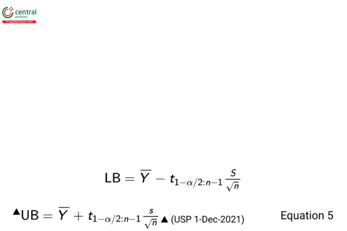
where n is the sample size and t_{1−α/2:n−1} is the 1 − α/2^th quantile of the cumulative Student t-distribution having area 1 − α/2 to the left and n − 1 degrees of freedom. One-sided intervals based on the individual bounds can be similarly defined.

The sampling and calculation process described above will provide a confidence interval that contains the true parametric value 100 × (1 − α)% of the time. Alternatively one can utilize a Bayesian approach to derive an interval which contains, with probability 100 × (1 − α)% the true value of the mean (12).

4 STUDY CONSIDERATIONS

There are a number of scientific and statistical considerations in conducting a study. These will be discussed in the context of the stages of the scientific method (see Introduction).

4.1 Study Objective

The study objective is a statement of the goal(s) of the study. Generally, the goals are placed into two categories: (1) estimation, and (2) inference. Estimation is the goal when the investigator wishes to report results that estimate true quantities that underlie the data generating process and are the subject of the study. In statistics these true quantities are called population parameters. Inference includes the additional step of using these estimates to make a decision about the unknown true value of the population parameter.

Numerical estimates can either be single numbers (point estimates), a range of numbers (interval estimates), or distributions (distributional estimates). A point estimate is a single number that “best” represents the unknown true value of a population parameter. The computed average or standard deviation of a data set sampled from the study population are examples of point estimates. “Best” in this context means the estimate is in some sense close to the unknown parameter value, although the difference between the estimate and the parameter will vary from sample to sample.

A point estimate reported alone has little utility because it doesn’t reflect the uncertainty manifested by the magnitude of the difference between the estimate and the true value. Statistical intervals can be used for this purpose. A discussion of statistical intervals can be found in 3. Basic Statistical Principles and Uncertainty, Basic Statistical Principles, Statistical Intervals. Interval estimates provide additional details that may be useful for risk based decision making.

Distributional estimates are used in Bayesian analysis to dene expectations when the population parameter is viewed as a random variable. In particular, posterior distributions formed by combining prior and sample information are used to assign probabilities that the unknown parameter will fall in a given range. Appendix 5: Bayesian Inference describes the utility of distributional estimates in more detail.

A statistical paradigm used to express the objective of an inferential study is a statistical hypothesis test. A hypothesis test is expressed as a pair of statements called the null hypothesis (H₀) and the alternative hypothesis (H_a). Both are expressed concerning some unknown population parameter. Population parameters are often denoted with Greek letters. The Greek letter theta (θ) will be used for illustration. A two-sided hypothesis test can be written as

H0 : θ = θ₀

Ha : θ  ≠ θ₀                     Equation 6

where θ₀ represents the hypothesized value for θ. The alternative hypothesis is sometimes called the research hypothesis because it represents the objective of the study. As an example, consider the true slope of a linear model representing the average change in the purity of a compound over time. Traditionally, this parameter is represented with the Greek letter beta (β). An investigator intends to determine if there is evidence that the average change in purity is a function of time. That is, if it can be shown that the true value of the slope is non-zero. Accordingly, Equation 6 is rewritten as

H₀ : β = 0                                   H_a : β ≠ 0            Equation 7

It should be noted that this is called a two-sided hypothesis because the direction of the difference is unspecified. This would be the case if the study sought to determine either a positive change (increase in purity) or a negative change (decrease in purity). But this is unlikely to be the desired objective of the study. It’s more plausible that the study would strictly seek to determine if there is evidence that average purity decreases over time. This would be expressed as a one-sided hypothesis test as follows

H₀ : β ≥  0

H_a : β < 0                     Equation 8

The choice of two-sided or one-sided hypothesis test should be made when formulating the study objective, and prior to design and execution of the study. It should be based on a plausible scientific objective and should never be decided on the basis of the study results. Examples of two-sided and one-sided hypothesis tests will be given in 5. Comparison of Analytical Procedures.

An additional consideration in formulating a study objective is the use of equivalence or noninferiority testing. These procedures require that the investigator formulate their hypotheses with a scientifically or practically meaningful objective. These will be illustrated in 5. Comparison of Analytical Procedures and is discussed in detail in Appendix 3: Equivalence and Noninferiority Testing.

4.2 Study Design

Study design should ensure an acceptable level of uncertainty in an estimation study or an acceptable risk for drawing the wrong conclusion in a test of inference. This can be managed through use of statistical design tools, including blocking and replication. As discussed previously, the design should also consider strategic selection of samples and study conditions which are associated with experiences in normal practice.

4.2.1 Design of an estimation study

The design of an estimation study may use suficient replication (sample size) and blocking to ensure desired control of the uncertainty in the result. To illustrate, consider estimation of a mean based on a simple random sample of n units from a study population. The half width of the confidence interval (also called the margin of error) in Equation 5 represents the uncertainty in the estimation of the mean. In planning the study, the margin of error can be defined to be no greater than a maximum allowable value H. Selecting the confidence level, (1 − α), and providing a preliminary estimate for the standard deviation (S), one can solve for a required sample size using the equation

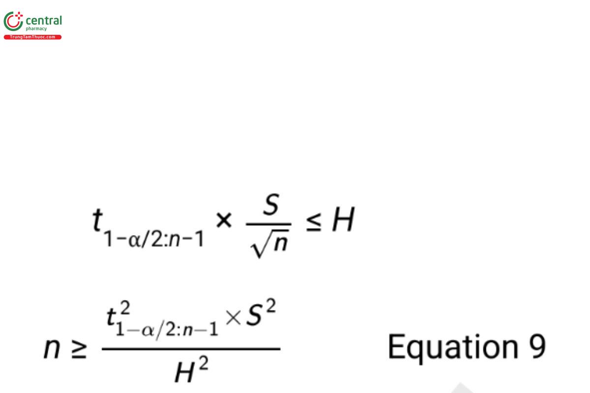
Since the degrees of freedom of the t-value are a function of n, one must either solve Equation 9 iteratively, or use an approximation by replacing the t-value with the associated Z-value. Preliminary estimates for S are obtained from similar studies or through the advice of subject matter experts. Scale of the data (e.g., transformed or original scale) should be defined prior to obtaining the preliminary estimate of the standard deviation or defining H (see Appendix 2: Models and Data Considerations for more on data transformation).

4.2.2 Design of an inferential study

The design of an inferential study is based on controlling the risks of drawing the wrong conclusion. Following the paradigm of a hypothesis test, these risks are illustrated in Table 1 and Table 2.

Table 1. Conclusions in a Statistical Test

Table 2. Probabilities of a Wrong Conclusion

It is important to determine the required sample size to control the Type I error (α) and Type II error (β) simultaneously. Formulas for sample sizes supporting an inferential study that depend on selected values of (α) and (β) are available in many textbooks and software packages. These formulas become more complex when the design includes blocking or experimental factors such as analyst or day. Computer simulation is a useful tool in these more complex situations, and support of a statistician can be useful. 

While replication is an effective strategy for reducing the impact of random variability on uncertainty and risk, blocking can be used to remove known sources of variability. For example, in a study to compare two analytical procedures, each procedure might be used to measure each sample unit of material. This results in the removal of the variability between sample units of material, which provides a reduced error term used to compare differences between the two procedures. By reducing the error term in this manner, the power of the experiment is increased for a fixed number of sample units. A numerical example is provided in 5. Comparison of Analytical Procedures. 

It is important to avoid introducing systematic error or bias into the study results. Bias can be introduced through unintentional changes in experimental conditions, due to either known or unknown factors. Effective sampling and randomization are important considerations in mitigating the impact of bias. Sampling is performed after the study has been designed and constitutes the selection of test articles within the structure of the design. How to attain such a sample depends entirely on the question that is to be answered by the data. When possible, use of a random process is considered the most appropriate way of selecting samples. 

4.3 Study Conduct

The most straightforward type of random sampling is called simple random sampling. However, sometimes this method of selecting a random sample is not desirable because it cannot guarantee equal representation across study factors. The design of a study to release manufactured lots might incorporate factors such as selected times, locations, or parallel manufacturing streams (e.g., multiple filling lines). In this case a stratified sample whereby units are randomly selected from within each factor can be utilized. Regardless of the reason for taking a sample, a sampling plan should be established to provide details on how the sample is to be obtained to ensure that it is representative of the entirety of the population of interest. 

Randomization should not be restricted to sampling. Study samples should be strategically entered into an analytical procedure using randomization, while blocking can be utilized to avoid confounding of the study objective with assay related factors. Sometimes it’s impossible to utilize sampling plans which are random or systematic in nature. This is especially true when the population is infinite. In this case representativeness is addressed through study design including blocking, where factors which are known to be the key structural components of the population are used to represent the finite population. 

The optimal sampling and analytical testing strategy will depend on knowledge of the manufacturing, analytical measurement, and/or study related processes. In the case of sampling to measure a property of a manufactured lot, it is likely that the sampling will include some element of random selection. There should be sufficient samples collected for the original analysis, subsequent verification analyses, and other supporting analyses. In the case of sampling to address a more complex study, representativeness should be addressed through strategic design. It is recommended that the subject matter expert work with a statistician to help select the most appropriate sampling plan and design for the specified objective. 

An additional consideration in the conduct of a study is data recording. Many institutions store data in a laboratory information management system (LIMS). That data may be entered to the number of significant digits (decimals) of the reportable value for the test procedure. While this practice is appropriate for the purpose of reporting test data (such as in a certificate of analysis or in a regulatory dossier), it is inappropriate for data which may be used for subsequent analysis. This is noted in ASTM E29 where it is stated “As far as is practicable with the calculating device or form used, carry out calculations with the test data exactly and round only the nal result” (1). Rounding intermediate calculated results contributes to the overall error in the nal result. More on rounding is included in General Notices, 7.20 Rounding Rules and in Appendix 2: Models and Data Considerations. 

4.4 Study Analysis 

The culmination of a study is a statistical analysis of the data, and a decision in the case of an inferential study. Simple summaries such as group averages and appropriate measures of variability, as well as plots of the data and summary results facilitate the analysis and communication of the study results and decision. Summaries should be supplemented with confidence intervals or bounds, which express the uncertainty in the summary result (see 3. Basic Statistical Principles and Uncertainty). Transformations based on either scientific information or empirical evidence can be considered, and screening for outlying values and subsequent investigations completed (see Appendix 2: Models and Data Considerations). 

Many common statistical analysis tools are found in calculation programs such as spreadsheets and instrument software. Software which is dedicated to statistical analysis and modeling contain additional tools to evaluate assumptions associated with the analysis tools, such as normality, homogeneity of variance, and independence. Those with limited or no statistical training should consult a statistician throughout the process of conducting a study, including study design and analysis. Their statistical skills complement the laboratory skills in ensuring appropriate study design, analysis, and decisions. 

The study considerations outlined in this section will be illustrated hereafter. 

Change to read: 

5 COMPARISON OF ANALYTICAL PROCEDURES 

It is often necessary to compare two analytical procedures to determine if differences in accuracy and precision are less than an amount deemed practically important. For example, General Notices, 6.30 Alternative and Harmonized Methods and Procedures describes the need to produce comparable results to the compendial method. Transfer of analytical procedures as described in Transfer of Analytical Procedures 〈1224〉 allows for comparative testing as an acceptable process. A change in a procedure includes a change in technology, a change in laboratory (called transfer), or a change in the reference standard in the procedure. 

For purposes of this section, the terms "old procedure" and "new procedure" are used to represent a procedure before and after a change. Procedures with differences less than the practically important criterion are said to be equivalent or better (see Appendix 3: Equivalence and Noninferiority Testing). This section follows the outline described in 4. Study Considerations highlighting the scientific method of (1) study objective, (2) study design, (3) study conduct, and (4) study analysis. 

5.1 Study Objective of a Procedure Comparison 

The study objective of a procedure comparison is to demonstrate that a new procedure performs equivalent to or better than an old procedure. There are two conceptual study populations: All future measurements made with the old procedure on a particular process, and all future measurements made with the new procedure on the same process. Each procedure is described in terms of the mean and standard deviation of the population of measurements. The mean and standard deviation of the reportable value of the new procedure are denoted by the Greek symbols μ_N and σ_N respectively. The subscript N denotes the “new” procedure population. The mean and standard deviation of measurements using the “old” procedure are denoted μ_O and σ_O respectively. These means and standard deviations are unknown, but conclusions concerning their potential equivalence or noninferiority (the new procedure is not inferior to the old procedure) are informed by estimates resulting from the experiment. Characteristics for comparison are most generally accuracy and precision across the range of the assay, and across conditions experienced during long term routine analysis. A risk analysis should be performed to identify such conditions. Discussion of accuracy and precision are found in 〈1225〉.

5.1.1 Accuracy

To compare accuracy of two procedures, one compares the procedure means. In particular, accuracy is compared using the absolute value of the true difference in means,

|μ_D | = |μ_N − μ_O |. Equation 10

The objective of such a study is to demonstrate that |μ_D | is less than a value deemed to be practically important, d. As an example, d may represent a numerical value that is small enough so that an increase in bias of this magnitude does not negatively impact decisions concerning lot disposition (i.e., conformance to specifications). The hypotheses used in an equivalence test are

H₀ : |μ_D| ≥ d

H_a :  |μ_D| <  d        Equation 11

(see Appendix 3: Equivalence and Noninferiority Testing).

Probably the most difficult aspect of conducting an equivalence test is determination of d. Typically, d is determined in partnership between the analytical chemist and the statistician based on combined manufacturing and scientific knowledge. Definitions of d vary across companies based on differing risk proles and experience. In some cases there exists a large amount of legacy data that may inform the decision, while in other cases there may be only limited data. An example where d is based on requirements of a manufacturing process follows in the section Determination of d and k.

5.1.2 Precision

To compare precision of two procedures, one compares the procedure standard deviations. Whereas a comparison of means involves a difference, a comparison of standard deviations involves the ratio

σ_N/σ_O            Equation 12

The study objective is to demonstrate that the ratio in Equation 12 is less than a practically important value k. The noninferiority hypotheses are

H₀ : σ_N/σ_O ≥ k

H_a :  σ_N/σ_O <  k          Equation 13

(see Appendix 3: Equivalence and Noninferiority Testing). The selection of k should be in alignment with the selection of d for the accuracy assessment. This process is demonstrated in the following section. 

5.1.3 Determination of d and k

Values of d and k for the tests of accuracy and precision should be internally consistent. To demonstrate, consider a case where historical measurements using an old procedure for a monitored process have a process mean of μ_O = 100 units and a combined process and analytical variance of σ²_L+ σ²_O = 0.80 where σ²_L represents lot-to-lot variability of the manufacturing process. Historic measurements of a reference standard provide the estimate σ²_O = 0.16 so that the assumed value of the lot variance is σ²_L = 0.80 − 0.16 = 0.64. The process specifications are the lower specification limit (LSL) = 96 units and the upper specification limit (USL) = 104 units. The same manufacturing process measured with the new procedure can be represented as having mean μ_N = μ_O + d and total process and analytical variance σ²_L+ σ²_N = σ²_L + k2σ²_O.

Kringle et al. (18) recommend selecting values of d and k consistent with a rule that states the proportion of product that falls outside of specification (OOS) when measured with the new procedure is acceptable. Table 3 reports the OOS rate when the process is in control and measured with the new procedure for several values of d and k. (Since the specifications are symmetric around μ_O , negative values of d provide the same OOS rates as the positive values shown in the Table 3).

Table 3. OOS Rate with New Procedure for Values of d and k

Table 3 assumes the process is normal and the probability (Pr) in any cell is given by the equation 

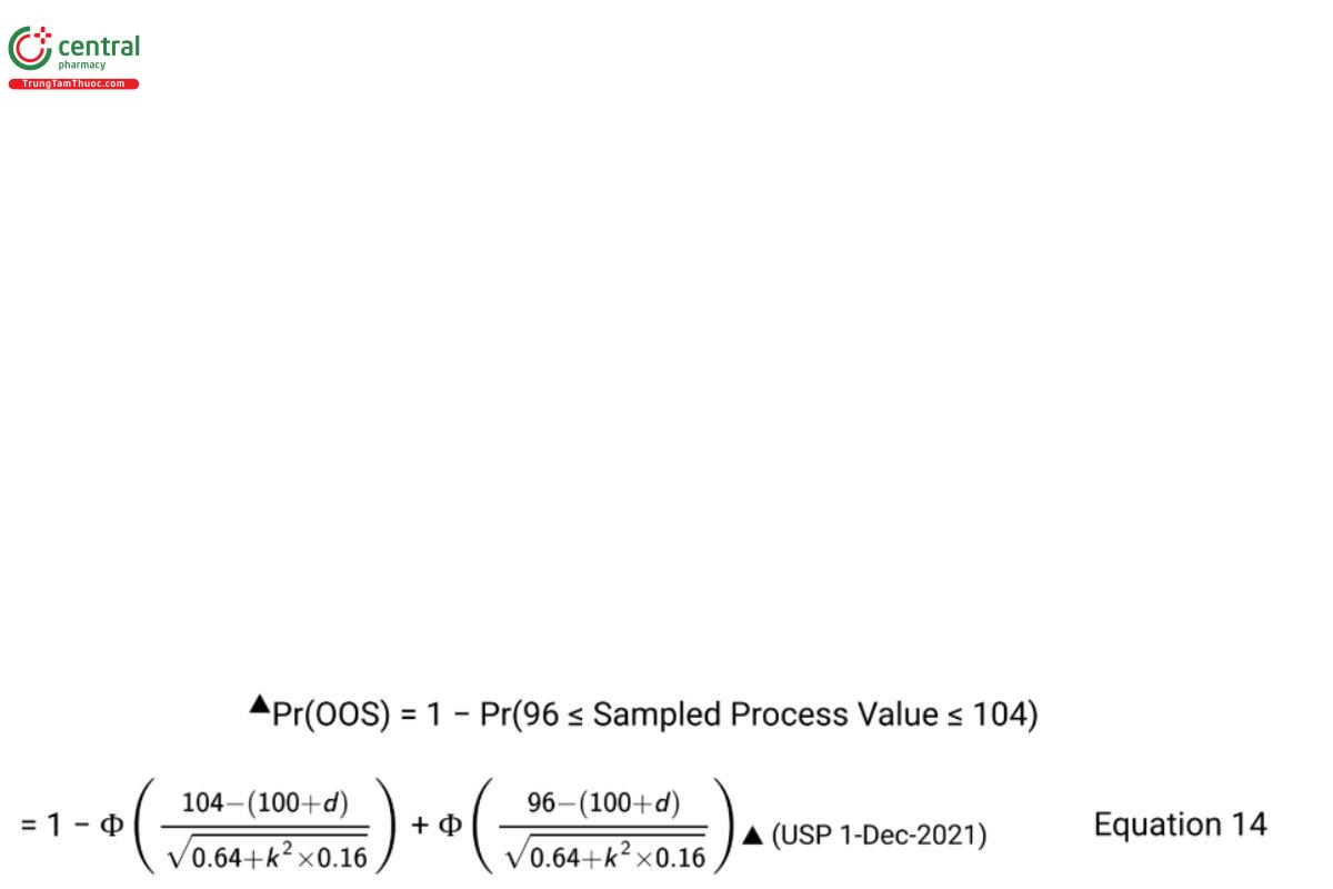
where Φ(●) represents the cumulative probability function of the standard normal distribution. The choice of OOS rate with the new procedure should be a business decision. (USP 1-Dec-2021)

5.2 Study Design of a Procedure Comparison

The study design for comparing the old and new analytical procedures is comprised of the selection of test materials, experimental design, and sample size determination (the so-called "power calculation"). Results for two scenarios are provided in this section. The rst scenario considers samples from homogeneous test material, and the second scenario considers test material with variation across sample units.

5.2.1 Scenario 1: homogeneous test material

In this scenario, test samples of homogeneous material are selected and measured using one of the procedures on each test sample. There are n_O samples measured with the old procedure and n_N samples measured with the new procedure. It is recommended to design the study so that n_O = n_N . Table 4 presents this design, which is referred to as an independent two-sample design.

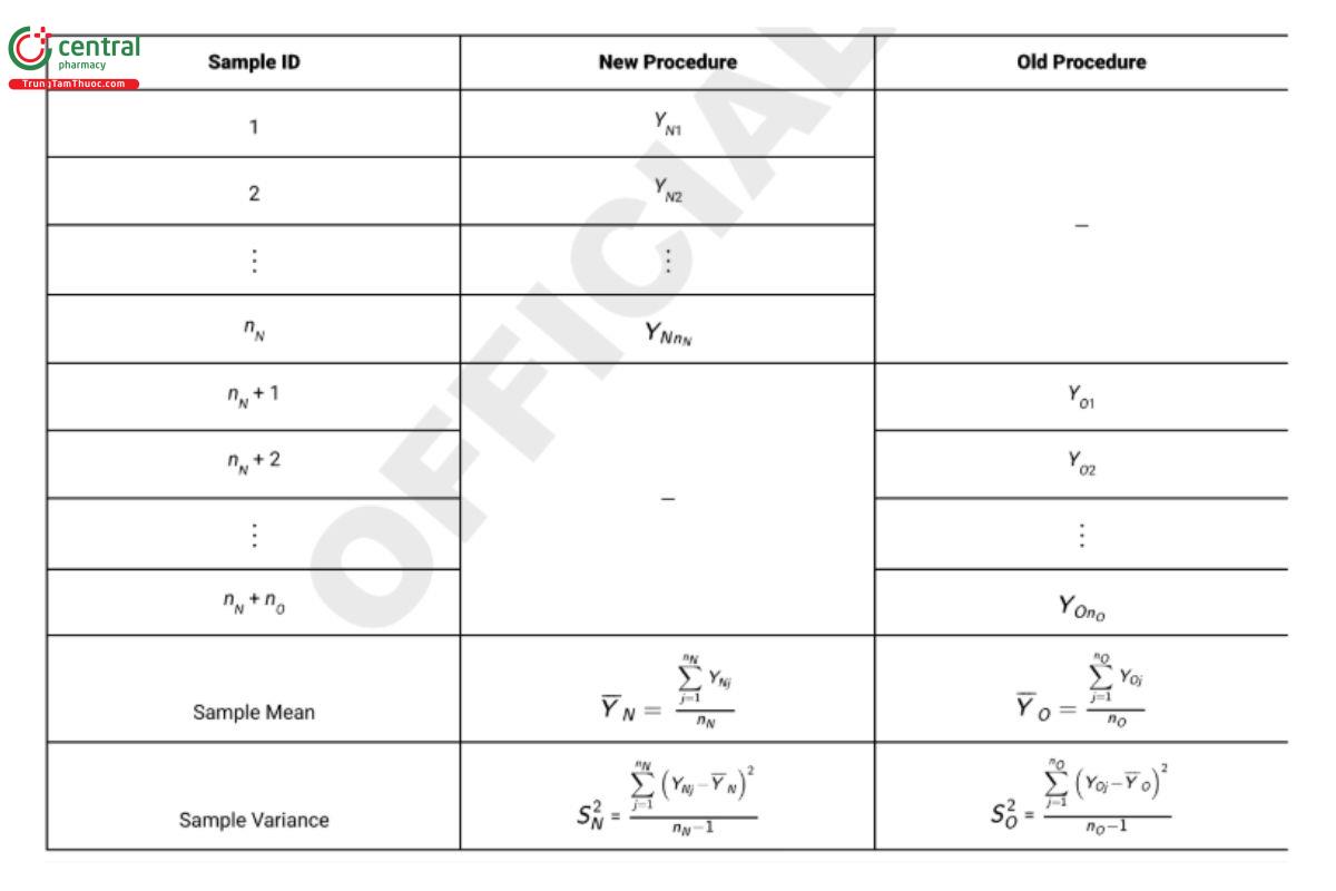
For the comparison of means the estimator of interest is the difference of sample means, Y_N − Y_O which has variance

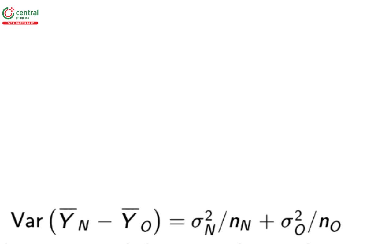
Power calculations are needed to ensure the sample size is great enough to find evidence that H is true when such is the case. For testing the equivalence hypotheses in Equation 11 assuming σ_N = σ_O , Bristol (8) recommends the sample size formula 

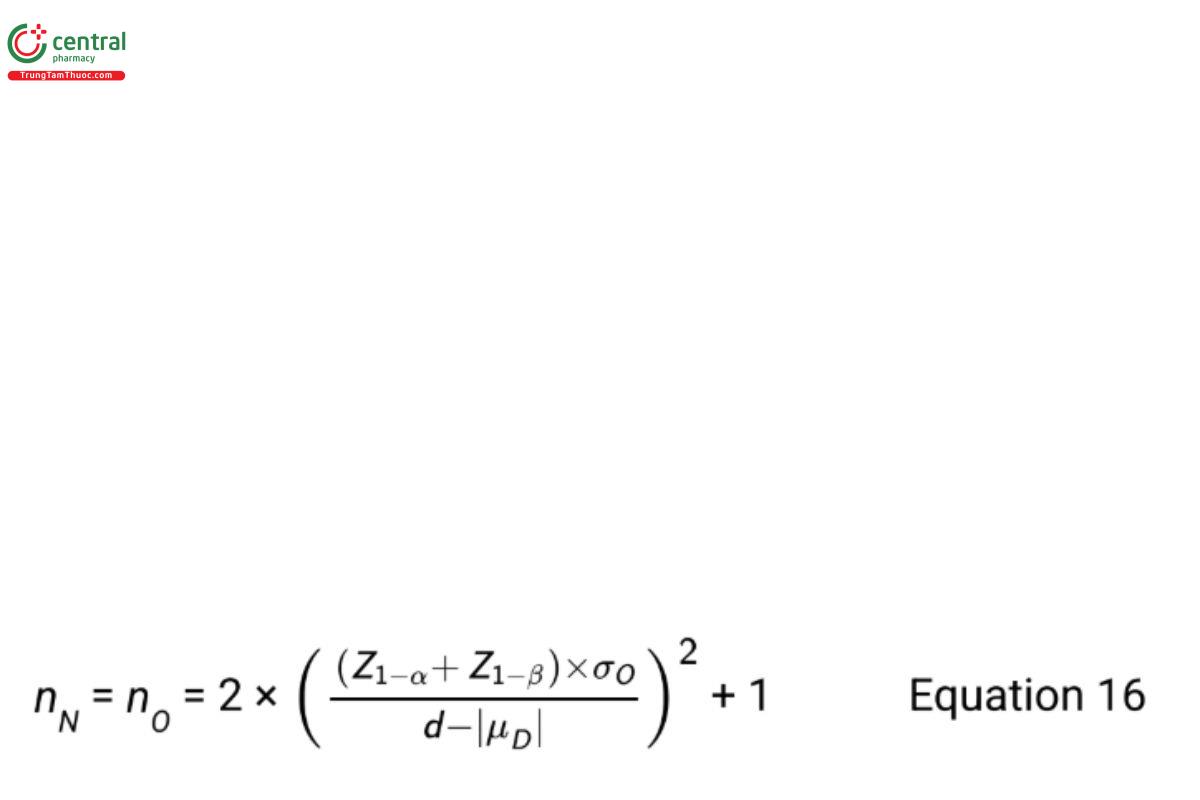
where Z_1−α and Z_1−β are standard normal percentiles with area 1−α and 1−β respectively, to the left. The Type I error rate is α and the Type II error rate is β. When |μ_D | is equal to zero, replace Z_1−β with Z_1−β/2 .

If it is desired to have a probability of passing of 85% (β = 0.15) with α = 0.05 when means differ by one standard deviation, i.e., with |μ_D |=σ_O = √0.16 = 0.4, and d=1, the required sample size for both the new and old procedures is given by the equation

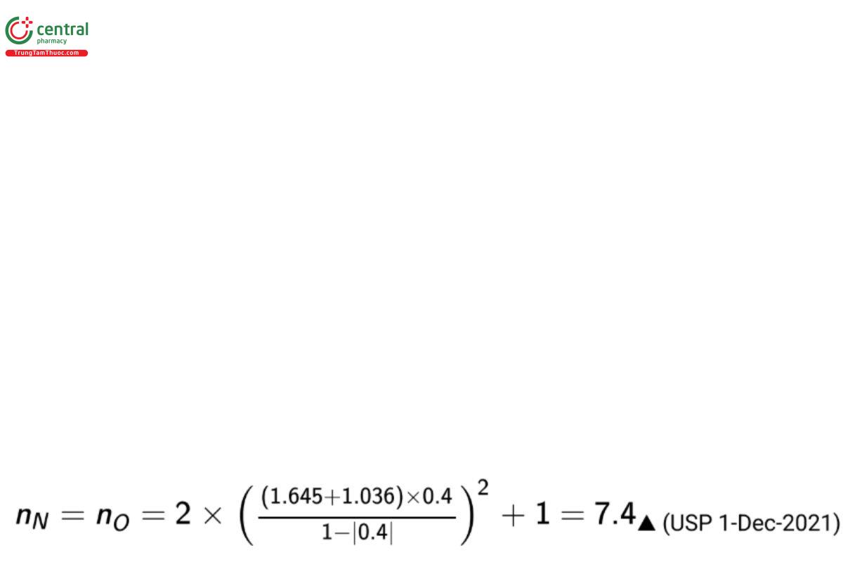
which is rounded up to 8 for each procedure (for 16 total test samples).

To test the noninferiority hypotheses in Equation 13, it is desired to have a high power when σ_N = σ_O .

The required sample size is obtained by solving for n_N and n_O iteratively using the equation

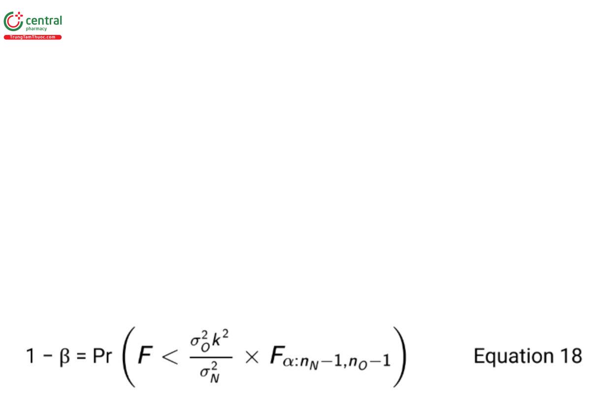
where F is a random variable following the F-distribution with degrees of freedom n_N − 1 and n_O − 1. As noted earlier, it is recommended that n_N = n_O (USP 1-Dec-2021) . Table 5 reports the power for sample size combinations with k = 2, (USP 1-Dec-2021) α = 0.05, and σ_N = σ_O = 0.4.

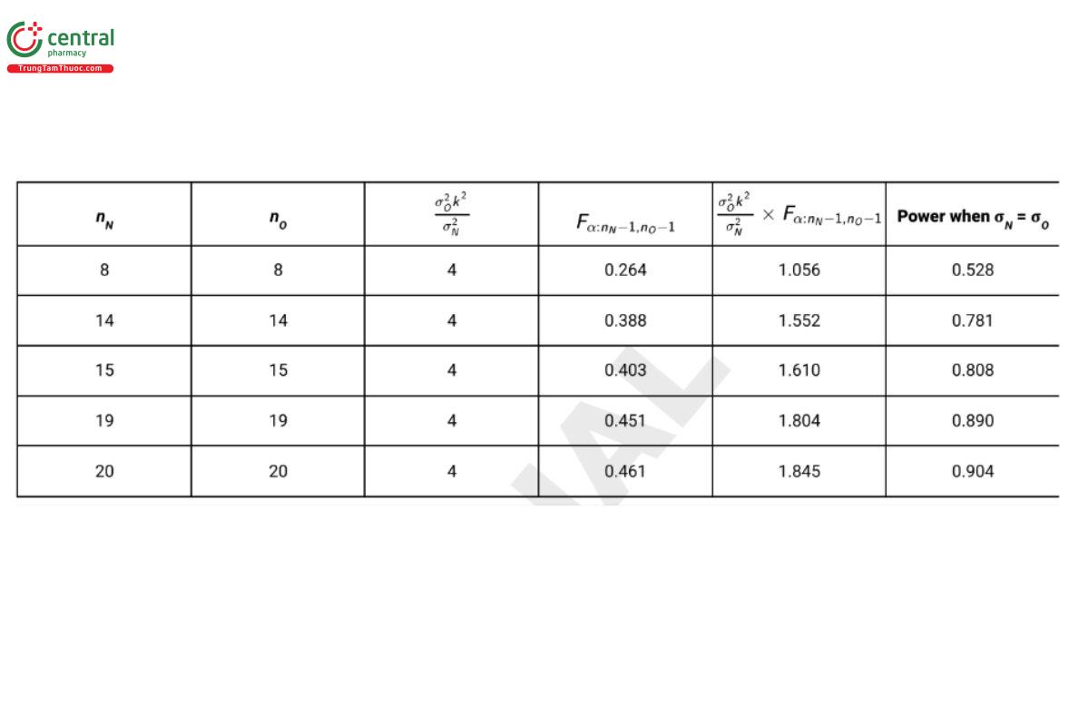
From Table 5 it is seen that the sample of size 8 required for the test of equivalence of means does not provide acceptable power for the noninferiority test (power = 0.528). This is because estimates of standard deviations have greater uncertainty than estimates of means. Practicality often dictates that one select a greater value for β in a test of noninferiority than in a test for equivalence of means. In the present example, β is selected as 0.20 in the test for noninferiority, and (USP 1-Dec-2021) a sample size of 15 per procedure (30 test samples in total) is selected for the design.

When a comparison is made between laboratories (as during procedure transfer) it’s important to keep in mind that in order to be representative of future testing, the study design should include factors which have significant impact on the long term performance of the procedure. As noted previously, this may include analyst, but may also require that multiple instruments and batches of key reagents be included in the design. These may be nested or crossed. Failing to do so may underestimate the variability or confound the effects of some factors with the difference between labs. In general factors such as analysts where levels are unique within each laboratory might be nested within each lab, while factors such as reagent lots which might be routinely shared across laboratories could be crossed with laboratory. As such, the estimates of variability used in these equations should be representative of the variability induced by these factors. The best estimates of variability come from data collected on samples tested across a broad period of time, such as stability samples and an assay control. More considerations of this nature are described in 〈1210〉.

5.2.2 Scenario 2: variation across test samples

It is often desirable to compare procedures across manufactured lots or use different manufactured levels of an analyte. This is important if the study objective is to ensure the range of the procedure in the new laboratory, or when the procedure is intended to measure degraded samples. This selection of test material introduces a new source of variation to Scenario 1 that must be considered during the study design in order to most efficiently compare the two procedures.

The recommended design in Scenario 2 is a paired design in which each test sample is measured independently by both procedures, instead of having each test sample randomly measured by only one procedure as in Scenario 1. The term “test sample” is referred to as a blocking factor because observations within the same block are differenced (see 4. Study Considerations). This has the effect of removing the variation across test samples from the analysis. Table 6 presents a schematic illustration of the paired design using n test samples.

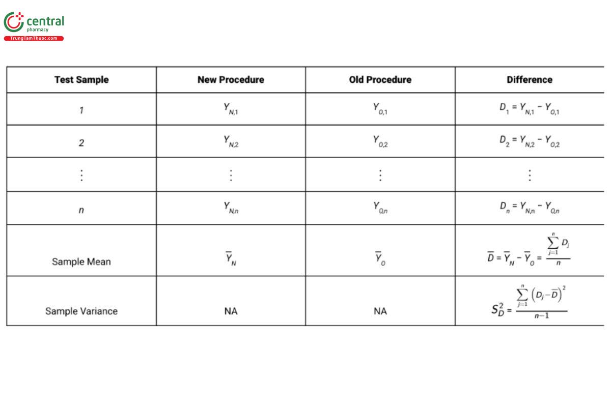
Using the paired design with n lots, the variance of D is ( σ²_N + σ²_O )/n because the variability due to lots disappears when results on the same lot are differenced. The unbiased estimator of σ²_N + σ²_O is S²_D . 

The sample size formula for satisfying the mean test requirements for a paired design (USP 1-Dec-2021) is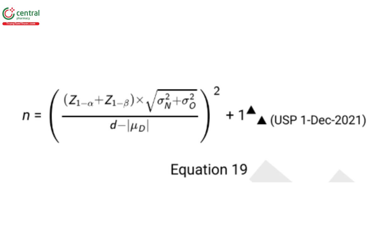 

(USP 1-Dec-2021) Using the same planning data from Scenario 1, d = 1, |μ_D | = 0.4, σ²_N = σ²_O=0.16, β = 0.15, and α = 0.05, the required sample size is

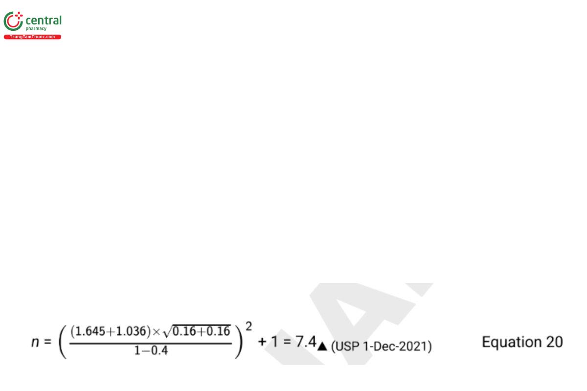
which is rounded up to 8 test samples (which are each measured once by each procedure). When using a paired design for the test of non inferiority, the ability to nd a good estimate of σ²_O is critical. Good estimates of σ²_O are often available from previous method validation studies or repeated measurements of an assay control. If no such estimate exists, it is necessary to modify the design in Table 6 and record two independent measurements with each procedure on each test sample. Independent estimates of both σ²_O and σ²_N can then be computed from the differences of the two paired values as shown in the section Study Analysis of a Procedure Comparison that follows. If a good estimate for σ²_O is available, the required sample size for the noninferiority test is derived iteratively from the equation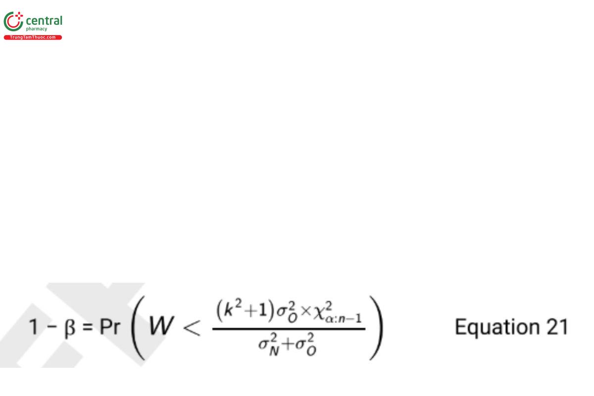

where W is a chi-squared random variable with n − 1 degrees of freedom. 

Table 7 reports the power for sample size combinations when α = 0.05,k=2, (USP 1-Dec-2021) and σ_N = σ_O = 0.4. 

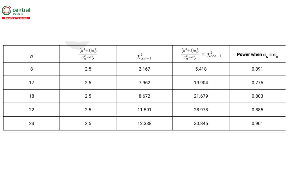
To obtain a power of 0.80 when the two standard deviations are equal, a sample of 18 test samples is required. Note that each test sample need not be unique. For example, if samples are being selected from three lots of product, one could select 6 test samples from each lot.

5.3 Study Conduct of a Procedure Comparison

When conducting the study, it is important to observe the random assignment of test samples to procedures in Scenario 1 in order to guard against possible bias. If repeated measurements are used in Scenario 2 to provide individual estimates of σ²_O and σ²_N, then independent measurements are needed. This will require independent preparations for each portion of the test sample.

5.4 Study Analysis of a Procedure Comparison

Two examples are provided to demonstrate the described formulas. Data in the examples were simulated from a population where μ_N = μ_O= 100 and σ²_O = σ²_N . These values were selected to demonstrate the computed sample sizes are suficient under the assumed conditions.

5.4.1 Scenario 1: homogeneous test material

Table 8 reports a sample data set with n_N = n_O = 15.

Table 8. Data from Simulated Two-Sample Independent Design

Accuracy is tested using the hypotheses in Equation 11 by constructing a 100(1 − 2α)% confidence interval on μ using the equation

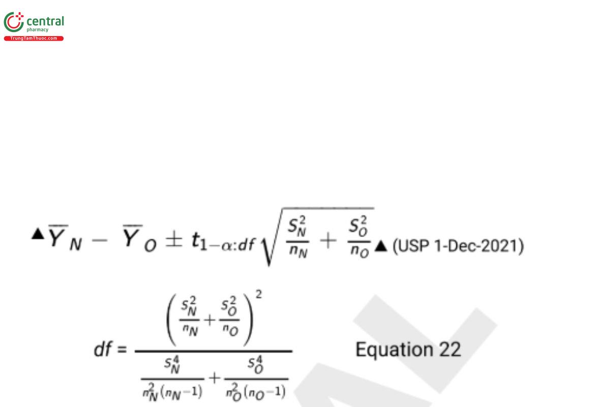
where t_1−α:df is a quantile from a central t-distribution with area 1 − α to the left and degrees of freedom (df). The null hypothesis in Equation 11 is rejected, and equivalence demonstrated if the entire confidence interval computed from Equation 22 falls in the range from −d to +d. This is the TOST described in Appendix 3: Equivalence and Noninferiority Testing and has a Type I error rate of α. With some software packages such as Excel, non-integer df-values are not accepted when determining the t-value. In this case, simply round to the nearest integer.

The 90% two-sided confidence interval that provides a Type I error rate of 0.05 computed from Equation 22 is

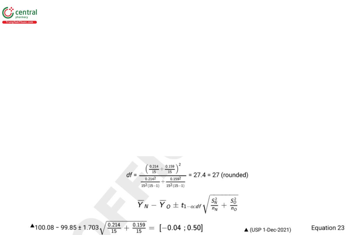
Since the computed confidence interval falls entirely in the range between −1 and +1 (i.e., −d to +d) equivalence of means has been demonstrated.

Precision is tested using the hypotheses in Equation 13 by constructing a 100(1 − α)% one-sided upper confidence bound on the ratio σ_N / σ_O using the formula

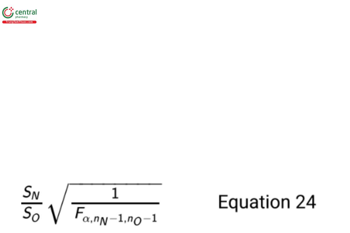
where F_{a,nN − 1,nO-1} is the F-quantile with area α to the left and degrees of freedom n_N − 1 and n_O  − 1 (USP 1-Dec-2021) . If the upper bound computed with Equation 24 is less than k, the null hypothesis is rejected and one concludes noninferiority of the standard deviation of the new procedure. This test has a Type I error rate of α.

The 95% upper bound on σ /σ computed from Equation 24 is

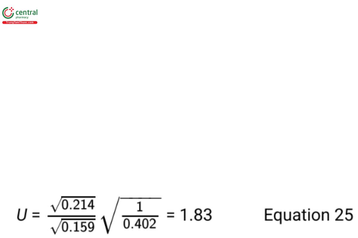
Since this upper bound is less than k = 2, noninferiority of the standard deviation of the new procedure has been demonstrated.

5.4.2 Scenario 2: variation across test samples

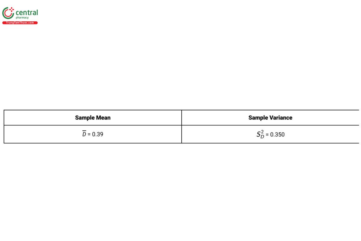
Table 9 provides summary results for 18 test samples in a paired design with D = Y_N − Y_O .

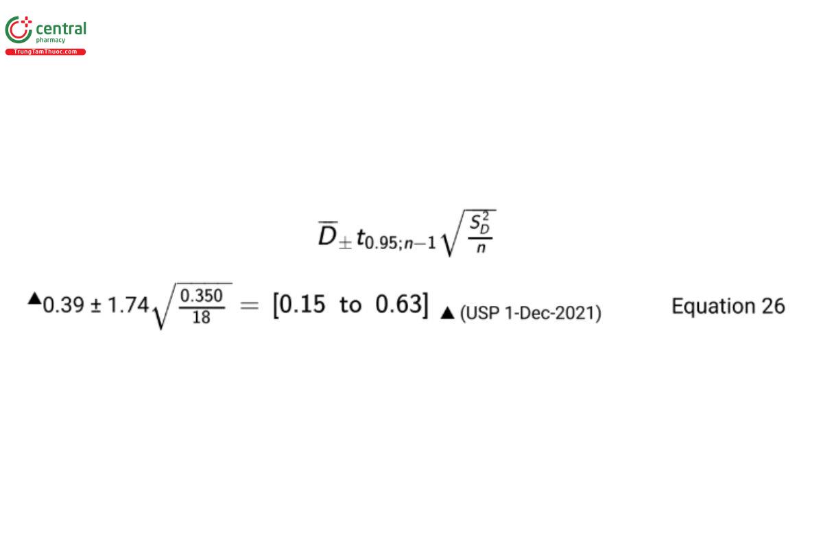
The 90% confidence interval on the difference in means for a paired design used to test equivalence of means with the data from Table 9 is

Since the computed confidence interval falls entirely in the range between −1 and +1 equivalence of means has been demonstrated. The noninferiority hypotheses in Equation 13 can be tested by constructing a 100(1 − α)% upper confidence bound on σ_N /σ_O using the formula

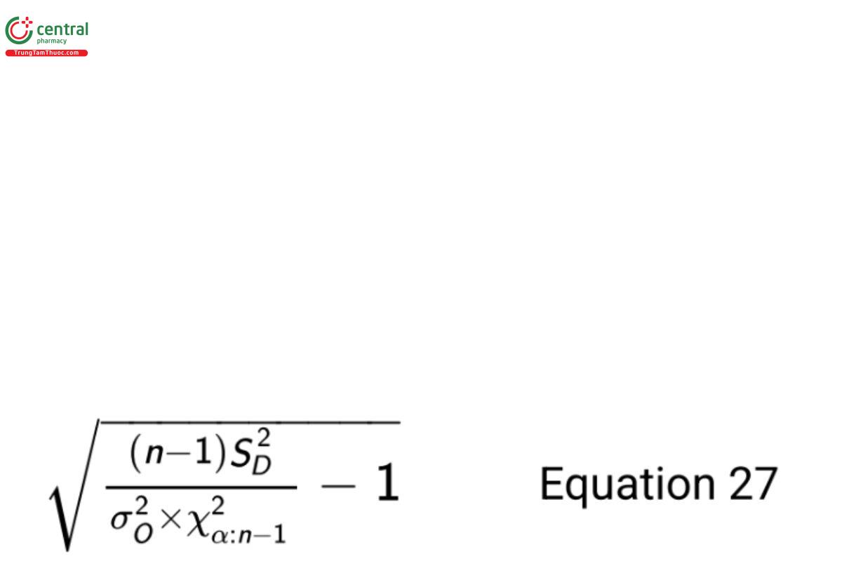
where X²_{α:n − 1} is a percentile from the chi-squared distribution with area α to the left and degrees of freedom n − 1. If this upper bound is less than k, the null hypothesis is rejected and noninferiority has been demonstrated.

From historical data used to plan the sample size, a good estimate of the old procedure variance is σ²_O= 0.16. Using the confidence bound in Equation 27, the 95% upper confidence bound on σ_N /σ_O is

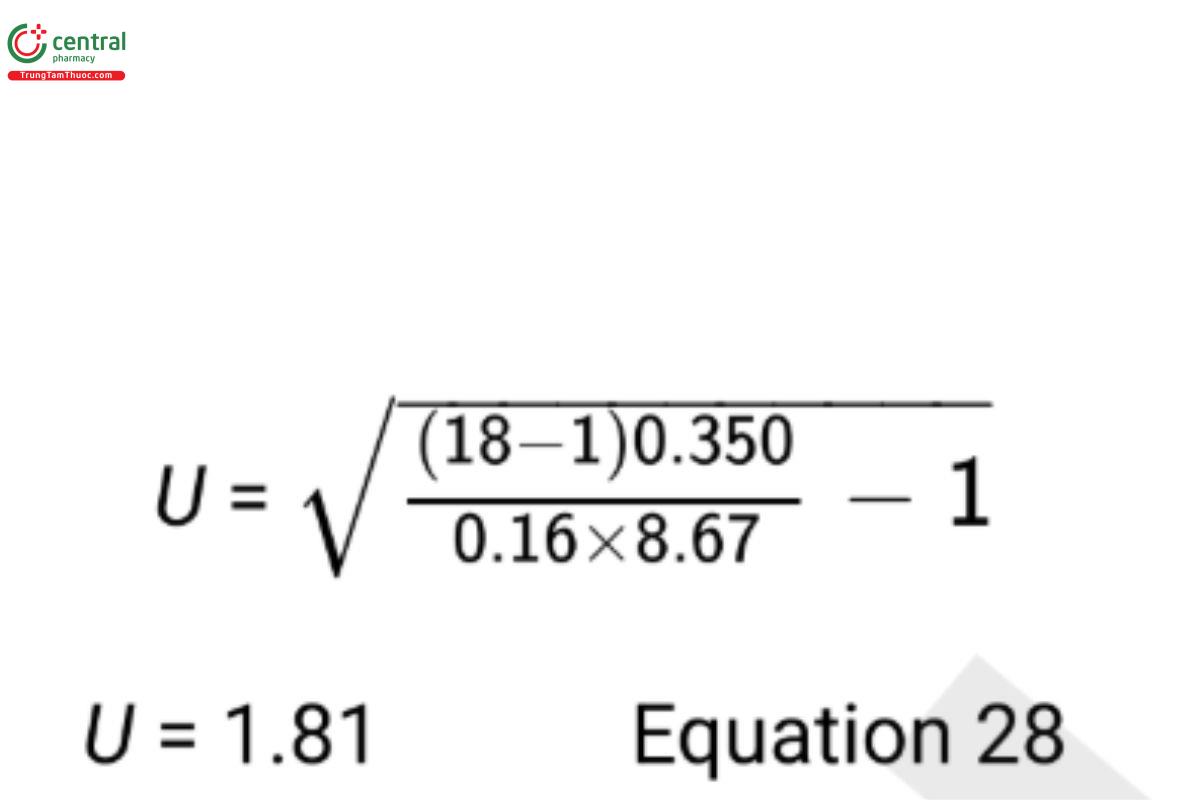
Since this upper bound is less than k=2, noninferiority of the standard deviation of the new procedure has been demonstrated. σ2O

If a good estimate of σ²_O is not available, the design requires replicate measures for each procedure on each test sample. Independent estimates of the analytical variances are computed using the formulas

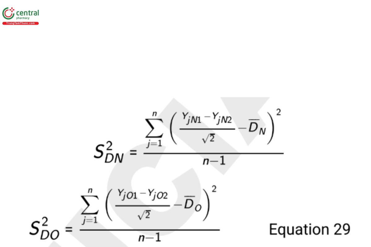
where Y_jN1 is the first measurement on test sample j with method N, Y_jN2 is the second measurement on test sample j with method N, Y_jO1 is the first measurement on test sample j with method O, and Y_jO2 is the second measurement on test sample j with method O. The resulting 100(1 − α)% one-sided upper confidence bound on the ratio σ_N /σ_O is

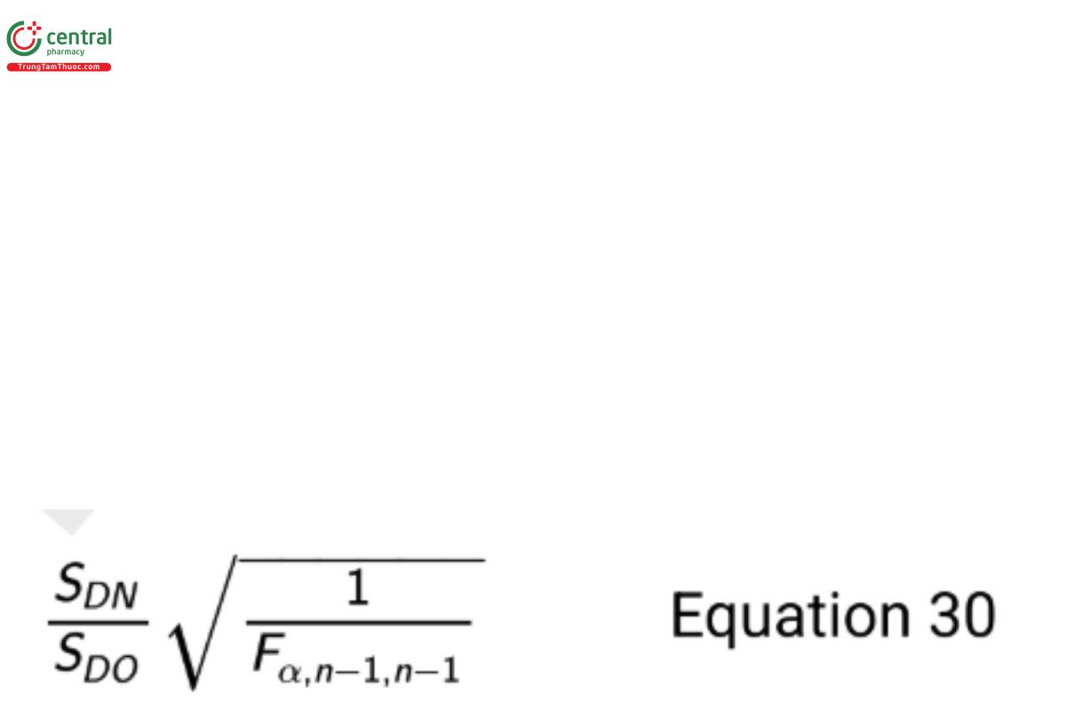
where F_{α/n−1/n−1} is the F-quantile with area α to the left and degrees of freedom n − 1 and n − 1, and n is the number of test samples (each with four independent measures). If this formulation is needed, then dene D_j = [(Y_jN1 + Y_jN2 ) − (Y_jO1 + Y_jO2 )]/√2 in the test for mean equivalence.

6 APPENDIX 1: CONTROL CHARTS

Control charts are used in the pharmaceutical industry to monitor the performance of manufacturing processes and analytical procedures. Using the vernacular of the scientific method, control charts are a tool to study these process populations, requiring a carefully developed objective, a strategic design, plans for implementation, and appropriate analysis. This appendix will discuss and illustrate the design and analysis of various control chart tools, as well as provide rules which are commonly used to make decisions.

Through its life cycle a process or a procedure can be influenced by known changes or unforeseen variability. For a manufacturing process this might impact the quality of the product or indicate the need to take action. For an analytical procedure which is routinely used to aid decision-making, this might increase the risk of drawing the wrong conclusion from a study or likewise indicate the need for action. Thus, it is important to continuously verify performance and provide ongoing assurance of a state of control. To this end, data from a manufacturing process or that relate to procedure performance are collected and analyzed. For a manufacturing process these may include process parameters and test results on manufactured materials. For an analytical procedure they can include analytical results for controls, standards used during the analysis, and system suitability data. It’s important to note that the control samples are used to monitor the performance of the procedure and are not an indicator of the product performance or characteristics (FDA ISO/IEC 17025 [21–23]). For purposes of this appendix the term "process" will be used to refer to both a manufacturing process and an analytical procedure.

Although various trending methods exist, control charts are one of the most simple and effective graphical tools for such analysis. There are many types of control charts including the following:

• Individual (I) chart for plotting individual values over time
• X-bar chart for plotting sample means over time
• Range (R) chart for plotting sample ranges over time
• Moving range (MR) chart for plotting moving ranges over time
• S-chart for plotting sample standard deviations over time
• Exponentially weighted moving average (EWMA) and cumulative sum (CUSUM) charts which are used when small shifts in the mean of the procedure are of interest

A typical control chart consists of a centerline and lower and upper control limits. The centerline represents the center of the distribution of a variable measured in the process. The two control limits are determined such that if the process performs as intended, nearly all results will fall within the two limits. Observations outside the limits or points within the limits that indicate a systematic or non-random pattern are indicative of a potential performance issue. Non-systematic patterns have been defined by WECO (which stands for Western Electric Company) and Nelson (20) that can be used in evaluating a control chart. Historical data (the “control data”) are typically used to obtain the centerline and lower and upper control limits. The control chart provides a visual means for identifying shifts, trends, and variability indicative of potential performance issues. A clarifying example is presented in the next section based on the Individual or I-chart.

6.1 Shewhart I-Chart

To develop a control chart for individual observations, it is customary to set control limits at

Process Mean ± 3 × Process Standard Deviation       Equation 31

These limits are based on assuming the process data follow a normal probability distribution and that a range of 3 standard deviations about the mean contains roughly 99.7% of all the data. Given a sample of Y₁, Y₂, … , Y_n observations from a controlled process, the process mean (average) is estimated using the formula.

The standard deviation can be estimated in a couple of ways, but for an I-chart, best practice is to base the estimate on the moving range statistic (MR). This estimator considers the “short term” variability of the process and guards against limits that are too wide if an unexpected trend exists in the data. Specifically, the MR represents the average difference of successive observations and is defined as

and the estimator for the process standard deviation is

where d₂ is a constant that depends on the number of observations associated with the moving range calculation (m). In Equation 33, m = 2 since the range is based on adjacent observations. The value of d₂ when m = 2 is 1.128. The upper control limit (UCL) and lower control limit (LCL) for the I-chart are then

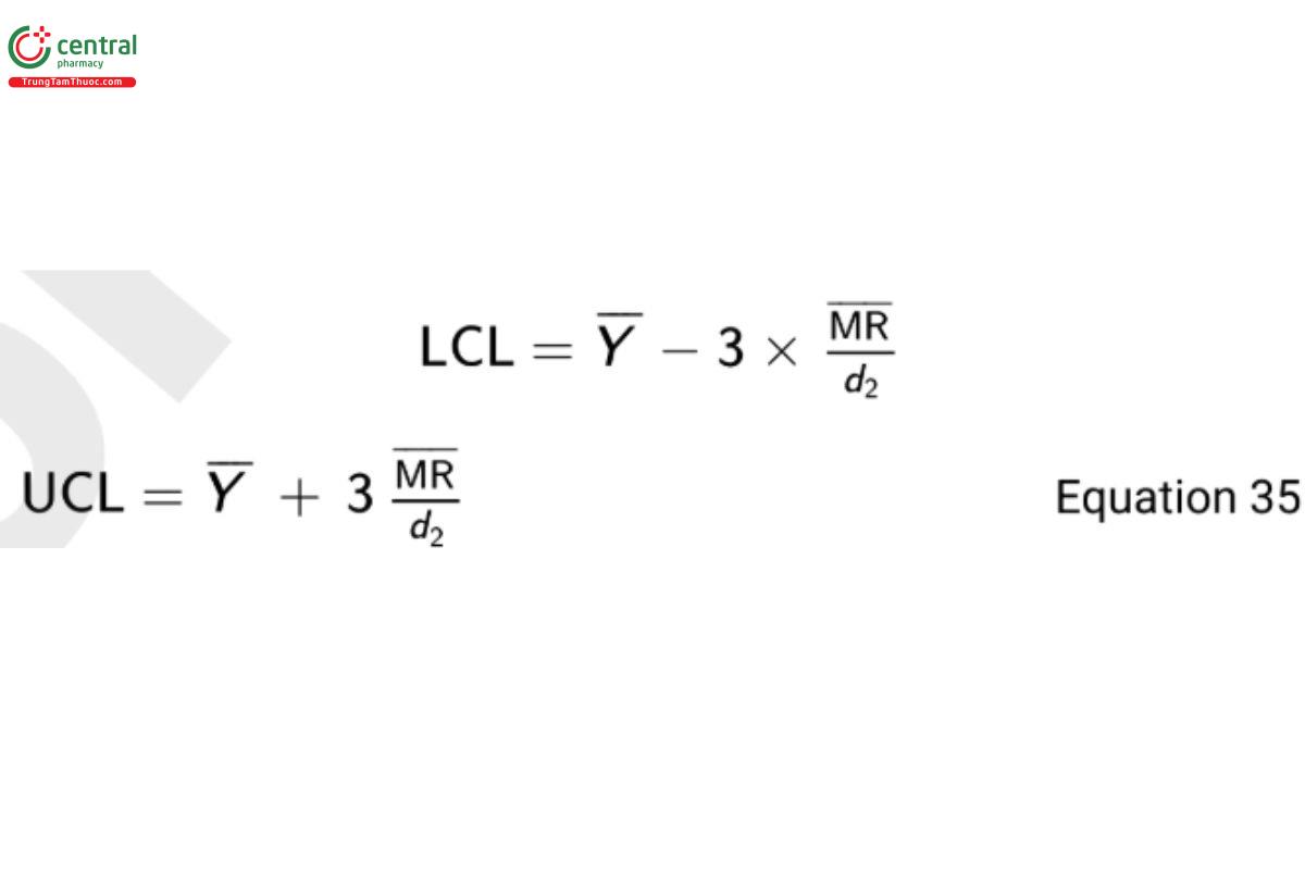
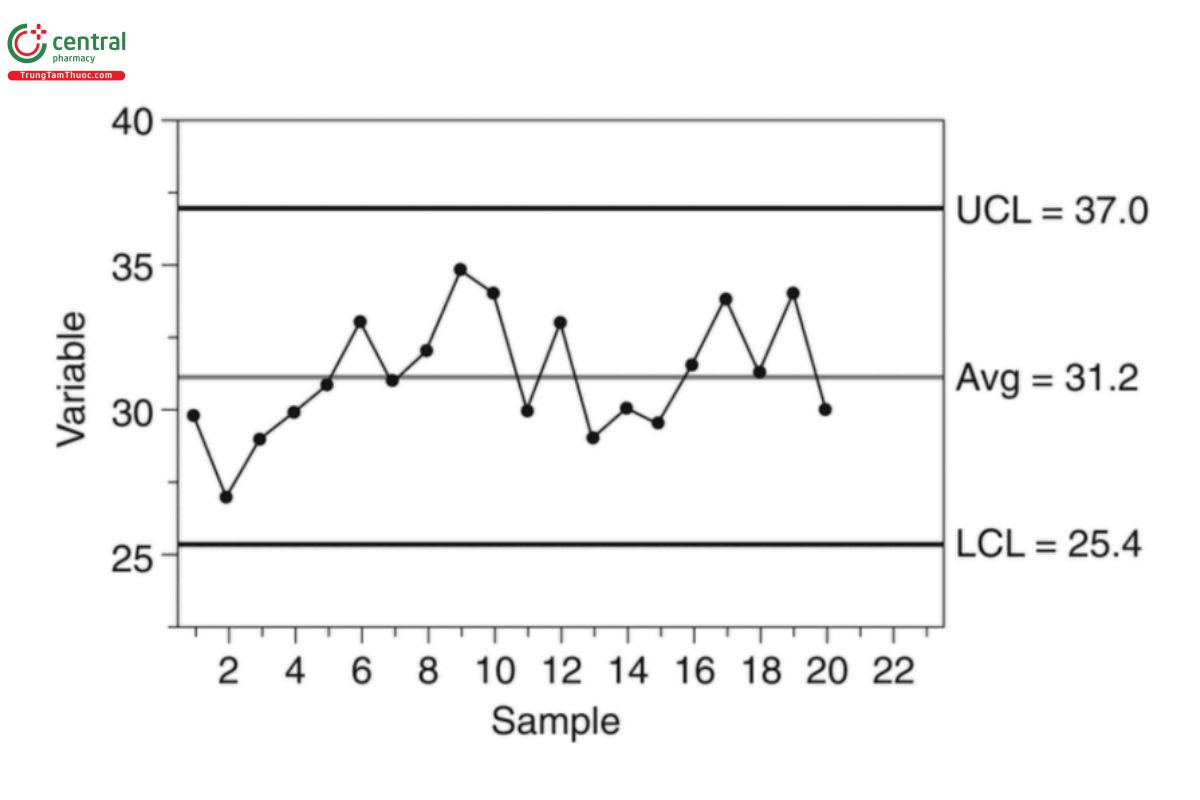
To demonstrate, consider a sample of 20 observations with Y = 31.2 and MR = 2.18. From Equation 35 the computed control limits are

LCL = 31.2 − 3 × 2.18/1.128 = 25.4
UCL = 31.2 + 3 × 2.18/1.128 = 37.0         Equation 36

The associated I-chart is shown in Figure 1.

6.2 Detection of Out-Of-Control Results

After a control chart is constructed, out-of-control results are detected using either WECO or Nelson rules. The Nelson rules are provided in Table 10. The relevance of these rules depends on the type of control chart. All eight rules can be applied to an I-chart, and selection of the particular rules depends on the desired sensitivity of the control process.

Table 10. Nelson Rules for Detection of Out-of-Control Results

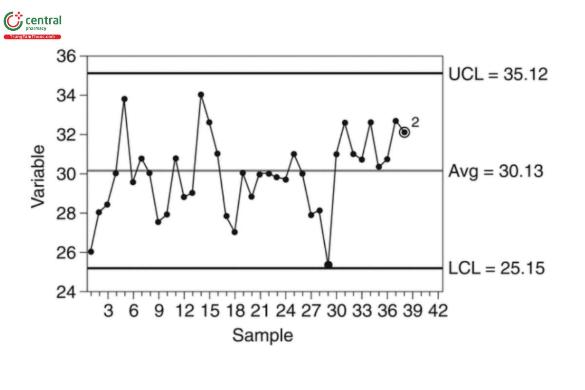
Figure 2 presents an I-chart for which a rule 2 violation is observed because the last 9 observations are all greater than the mean.

ASTM E2587 (3), Montgomery (19), and Wheeler (29) provide references for numerous control charts and example applications. Change to read:

7 APPENDIX 2: MODELS AND DATA CONSIDERATIONS

Statistical analysis involves models and assumptions associated with the reliability of fitting models to data. Models can be simple (e.g., a means model associated with a reportable value) or complicated (e.g., a nonlinear mixed effects model common in complex pharmaceutical settings). Assumptions monitored with residuals from the model t include normality, constant variance, and independence. This appendix focuses on adequacy of models that are t to analytical data, as well as data considerations such as significant digits, transformations, and outliers.

7.1 Models

In statistics, a model represents a functional description of some property(s) of a population. The term "population" refers to the set of all possible values of an attribute. A model parameter, also referred to as a population parameter, is the true but unknown value of a property, which is typically the subject of the statistical inquiry.

A means model characterizes the center of a univariate population, and can be written as

Y_i = μ + E_i    Equation 37

where Y is the ith observation in a sample of size n from the population, μ is a model parameter representing the population mean, and E the i i error. This error represents the effect of all factors that explain why the measured value is not always equal to μ. Such factors typically include lot-to-lot variation in product or analytical method error. The means model is the basis of statistical inquiries related to a population mean, usually estimated by the sample mean

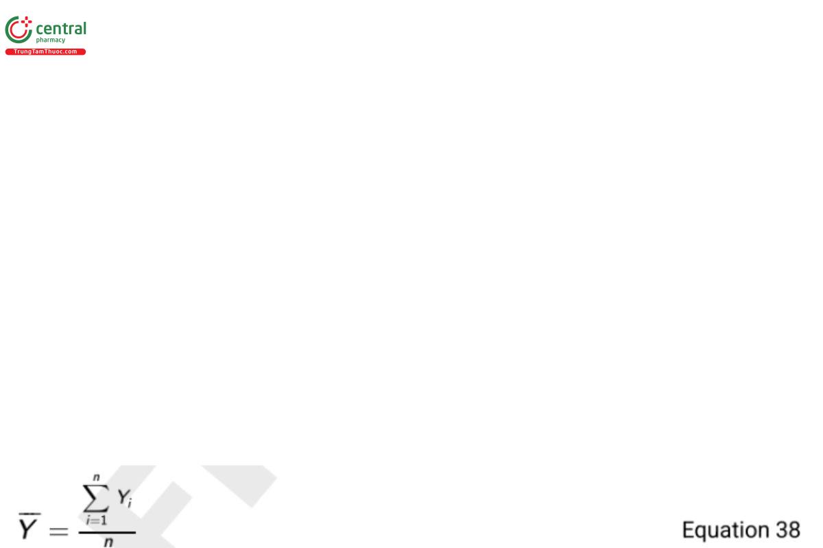
with errors estimated by residuals R_i = Y_i − Y.

Another familiar model is the simple linear regression model. This model characterizes the linear trend in the population mean with some covariate X (e.g., time or dose), and can be written as

Y_i = α + βX_i + E_i        Equation 39

where (X_i , Y_i ) is the ith observation in a sample of size n from the bivariate population, the parameters α and β are the intercept and the slope, respectively, that denes the functional relationship and E_i the error. Note that μ in Equation 37 has been replaced with α + βX_i in to allow the mean to change as a function of X_i. The parameters α and β are estimated from sample data as was in Equation 37. 

More complex models might be nonlinear, can include qualitative factors (e.g., analysts in a validation), or might include covariables which are random rather than fixed values (e.g., another measurement Z_i made together with X_i ).

7.2 Significant Digits

The number of digits used for calculations and the number of digits appearing in a reportable value should be considered separately. It's important to record and carry more digits during calculation than will be reported. It is a good practice to perform all statistical calculations with as many digits as practical. Rounding should be used only as a nal step before reporting the result. Automation facilitates the acquisition of numerous digits, while databases should be designed to store data with enough digits in anticipation of further calculations from the data.

The number of digits reported can sensibly be based on the standard deviation of the reportable value. ASTM E29, USPGeneral Notices, 7.20 Rounding Rules, and the FDA Laboratory Manual of Quality Policies (21–23) provide guidance on rounding and determination of sigfinicant digits in a reported value.

7.3 Transformation

A transformation is a functional re-expression of a measurement in order to better represent a known scientific relationship or to satisfy the assumptions of a statistical model. Transformations can also be discovered empirically with a representative set of the data using residual plots. One particularly useful transformation with analytical data is the logarithmic (log) transformation described in the next section.

7.3.1 log transformation

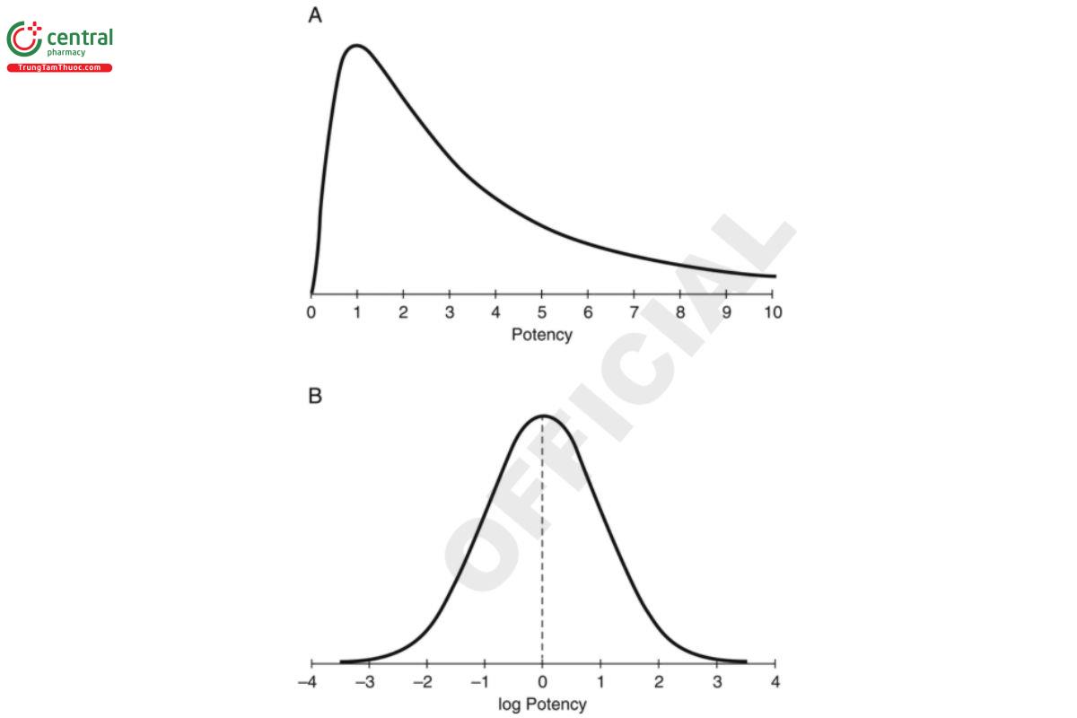
Examples of transformations using scientific knowledge of the measurement system come from many biological systems. In particular, variation around the responses predicted by a means model is often proportional to the response. For these systems, it is useful to work with the log of the original response which will have nearly constant variance across the range of the response. The shape of the transformed distribution will also be more symmetric as shown in the lower panel of Figure 3. A log transformation can be conducted using any base including Napierian (base e), common (base 10), or base 2.

Another reason for using a log transformation is that it can change a nonlinear functional form in the original scale to something more easily modeled in the log scale. For example, a log transformation can be used to re-express a nonlinear first order kinetics model as a linear model.

Statistical measures associated with the center and the dispersion from a sample are described in 3. Basic Statistical Principles and Uncertainty. These include the sample mean (Y) the sample standard deviation (S). These measures are meaningful when the data are approximately normally distributed and free of outliers. These measures may not be as meaningful when the normal distribution is not a good description of the data. To demonstrate, the top distribution in Figure 3 is skewed to the right. The greater values in the tail have the effect of pulling the mean to the right of where some would deem to be the “center” of the data. The lower distribution in Figure 3 shows the log-transformed responses of the top distribution. The top distribution is called a log-normal distribution because the distribution of its log values is normal. Because of the symmetry of the normal curve, the sample mean and sample standard deviation are meaningful estimates of the center and dispersion of the transformed distribution.

The sample mean of log-transformed responses can be transformed back to the original scale. This back-transformation results in what is called the geometric mean (GM) on the original scale. More formally, let Y_i represent a measured response on the original scale and T_i the transformed value of Y_i.

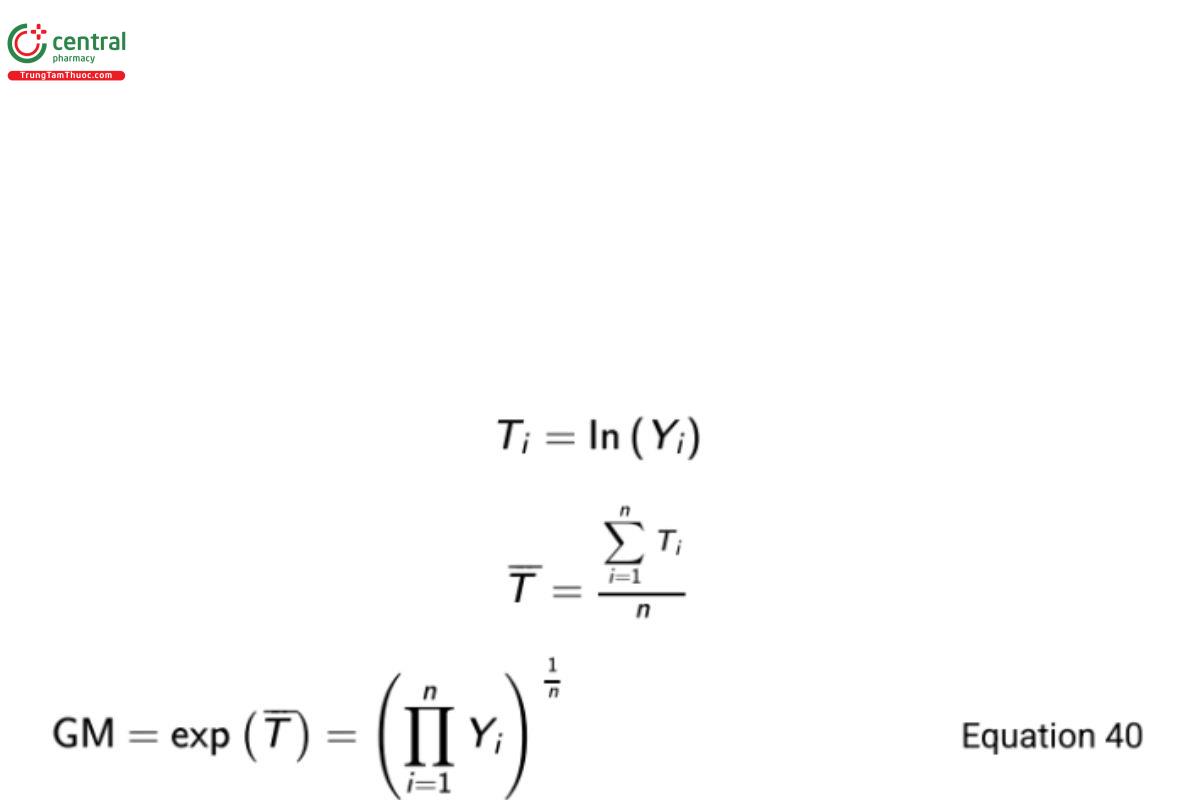
Then The standard deviation of log-transformed responses (S_T ) can likewise be back-transformed as exp(S_T ). This term is referred to as the geometric standard deviation (GSD) by Kirkwood (17). That is,

GSD = exp(S_T) Equation 41

Because S_T is non-negative, GSD ≥ 1 and represents a fold-variation in the response scale. While a summary for arithmetically scaled responses can be written as ± S, this might be summarized as GM ×/÷ GSD, or GM/GSD to GM × GSD for geometrically scaled responses. If for example GSD = 1.25 and GM = 1.0, a range might be summarized as 1.0/1.25 = 0.80 to 1.0 × 1.25 = 1.25. It should be noted that this represents a 1-standard deviation range. A more appropriate range might be calculated in the log transformed scale (see below). Kirkwood also denes the percent geometric coefficient of variation as

%GCV = 100 × (GSD − 1)%    Equation 42

An alternative measure of variability derived from the arithmetic moments of the log-normal distribution in the original scale is 

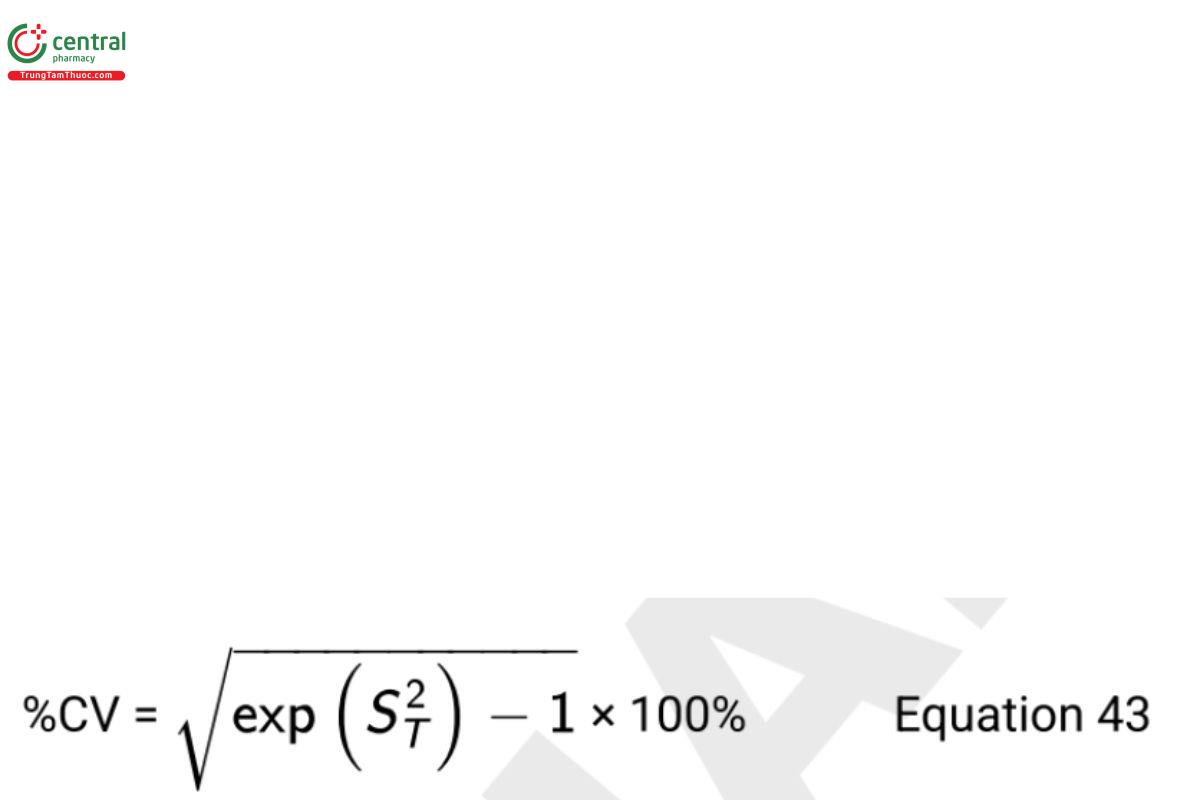
Numerically, %GCV and %CV of the log-normal distribution are close to each other when both are less than 20% (see Tan [25]). Their use along with GSD should be clearly specified when reporting the measure of variability or intervals for log-normal data. Interpretation of these measures are described more fully in Biological Assay Validation 〈1033〉, Appendices, Appendix 1: Measures of Location and Spread for Log Normally Distributed Variables.

From Equation 5 in 3. Basic Statistical Principles and Uncertainty, a 100(1 − α)% two-sided confidence interval on the mean in the log scale is

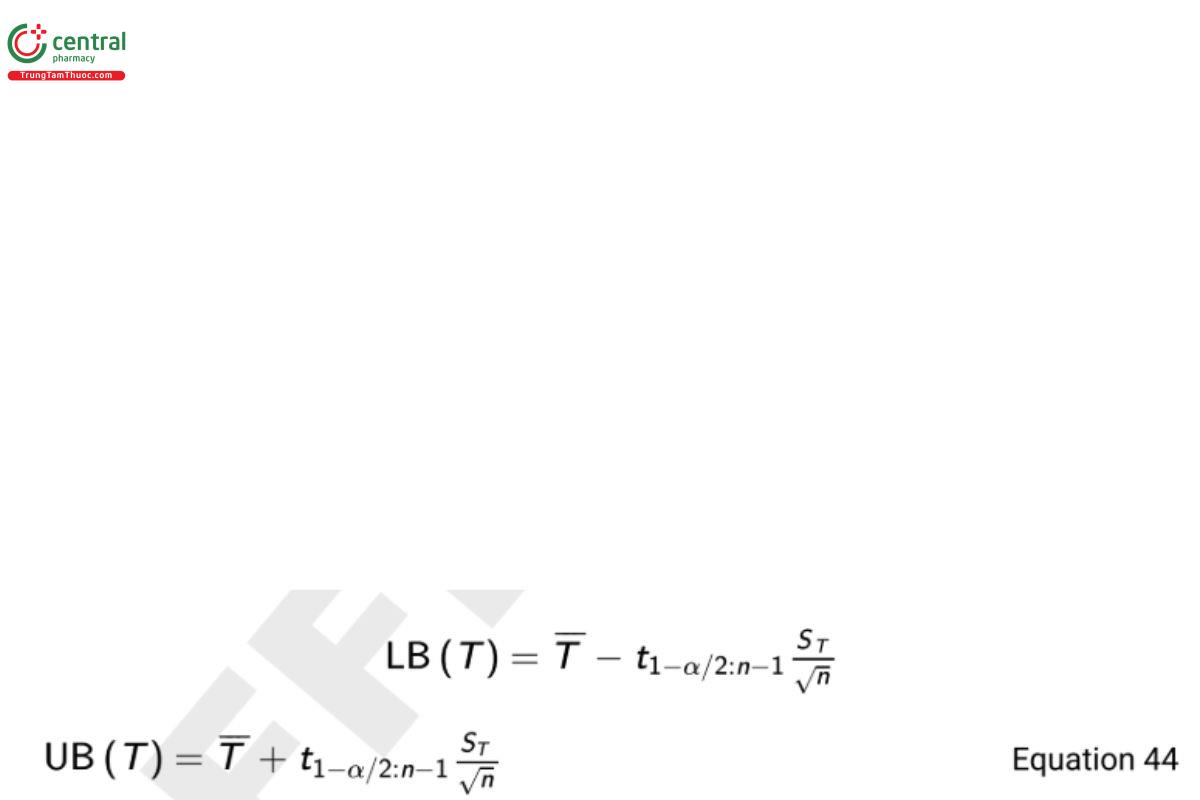
where n is the sample size and t_{1−α/2:n−1} is the 1 − α/2th quantile of the cumulative Student t-distribution having area 1 − α/2 to the left and n − 1 degrees of freedom.

The confidence interval on the geometric mean in the original scale is obtained from the bounds in Equation 44 as

LB(Y) = exp(LB(T))

UB(Y) = exp(UB(T)).        Equation 45 

Transformations other than logarithms may be considered for other types of data. For example, when working with proportions between 0 and 1 (or percentages between 0% and 100%), either the arcsine or logit transformation is useful. The arcsine transformation where Y is represented as a proportion is 

T = 2 × sin−1(√Y )         Equation 46 

and the logit transformation is 

T = ln (Y/(1-Y))          Equation 47

These transformations are particularly useful when a majority of the data are pushed against the upper bound of 1.0 or the lower bound of 0.0. Count data may be transformed using a square root or a log transformation of the count.

Power transformations, the most common of which are Box-Cox transformations, are also useful re-expressions. These transformations are of the form

T=(Y^λ-1)/λ          λ ≠ 0

= ln(y) λ = 0           Equation 48

where λ is selected to best transform the data set to normality. Information on Box-Cox transformations is provided in Section 6.5.2 of the NIST/SEMATECH e-Handbook of Statistical Methods (24).

Regardless of the transformation, summary measures and intervals calculated in the transformed scale can be back-transformed to the original scale. In all cases the data should be examined to establish if the transformed measurements exhibit almost uniform variability and are approximately normally distributed.

7.4 Assessing Model Adequacy

All models involve assumptions about the processes that generate the data and the data itself. In addition to the assumed functional form, the distribution of the error term in Equation 37 and Equation 39 is of primary importance. Typical assumptions are that the error terms are independent, normally distributed, and have constant variance across the range of responses. When these assumptions are reasonable, statistical models are usually readily interpretable and powerful (i.e., able to measure subtle effects with good precision and discrimination between groups). As attractive as any model might be, it is imperative to check for and address violations of the assumptions upon which these models rely. Assessing model adequacy is the process of verifying these assumptions.

There are both graphical and quantitative methods for assessing model adequacy. In many data analysis projects, there are multiple iterations of conversations between researchers and statisticians before selecting a nal model. Topics to consider include appropriate transformations of the data, the treatment and design factors of interest, potential candidate models, and assessment of model t.

Useful tools for assessing model t include residual plots with both raw and studentized residuals, model-based outlier detection methods, and regression leverage and influence measures. Plots of residuals can be generated in several ways. The most common format is a plot of the residuals on the vertical axis, and the predicted response on the horizontal axis. When the observations on a residual plot increase or decrease in spread along the horizontal axis, this indicates violation of the assumption of constant variance. Any linear or nonlinear trend in the residuals suggests the functional form of the model may not be correct, or that an important treatment factor is missing from the model. For example, a curved residual pattern may indicate the need for a quadratic term in the model. Additionally, residuals that fall outside the general cluster of points may be an indication of an outlier. As noted previously, some of these problems may be mitigated with an appropriate transformation.

Normality of the error terms is an especially important assumption if the model is used to predict future behavior. Graphical methods that can be used to monitor this assumption include dot plots, box and whisker plots, and normal probability plots (sometimes called quantile quantile plots or QQ plots). These graphical tools are available in many common statistical software packages. Statistical tests of normality are described in Section 1.3.5 of the previously referenced NIST handbook and available in statistical software packages.

Lack of independence typically occurs when data are in some manner “batched” in groups. For example, measurements that are taken from the same plates on an assay are more similar than measurements recorded on other plates. This so-called "intragroup correlation" can be properly modeled by including a “batch” factor in the model to account for the correlation.

Care should be taken in the assessment of model assumptions. Statistical tests in particular are impacted by the size of the sample. For small samples such tests may be insensitive for detecting departures from the model assumptions. In contrast for large samples, they may detect an assumption violation even though visual assessment suggests the assumptions are reasonable. A combination of scientific understanding of the measurement process generating the data, graphical analyses and statistical tests can be used together to address model adequacy.

7.5 Outliers

Occasionally, observed analytical results are very different from expected analytical results. Aberrant observations are properly called outlying results. These outlying results should be documented, interpreted, and managed. Such results may be accurate measurements of the property being measured but are very different from what is expected. Alternatively, due to an error in the analytical system, the results

may not be typical, even though the property being measured is typical. A first defense against obtaining an outlying analytical result is application of an appropriate set of system suitability and control rules (see Appendix 1: Control Charts).

When an outlying result is obtained, systematic laboratory and process investigations are conducted to determine if an assignable cause can be established to explain the result. Factors to be considered when investigating an outlying result include human error, instrumentation error, calculation error, and product or component deficiency. A thorough investigation should consider the precision and accuracy of the procedure, the USP or in-house Reference Standard and controls, process and analytical trends, and the specification limits. If an assignable cause due to the analytical procedure can be identified, then retesting may be performed on the same sample, if appropriate, or on a new sample. Based on the documented investigation, data may be invalidated and eliminated from subsequent calculations.

“Outlier labeling” is informal recognition of outlying results that should be further investigated with more formal methods. Outlier labeling is most often performed visually with graphical techniques such as residual plots, standardized residual plots, or box and whisker plots. “Outlier identification” is the use of statistical significance tests to confirm that the values are inconsistent with the known or assumed data distribution. The selection of the correct outlier identification technique often depends on the initial recognition of the number and location of the values.

A simple example is presented to demonstrate this process. An analytical procedure requires measurements from 3 vials of liquid drug product which are used to provide a reportable concentration value (mg/ml) for the lot from which the vials were selected. When measuring the third vial, the analyst noted a slight deviation in the sample preparation which was not discussed in the protocol. The three measurements are reported in Table 11. Vial 3 is the vial in question.

Table 11. Concentrations for 3 Vials of Drug Product

The residual plot for the mean model described in Equation 37 is shown in Figure 4. Here the residual is the measured value minus the sample mean of the 3 vials (50.5 mg/ml).

The residual for vial 3 visually resides far from the other two values and is accordingly labeled as an outlier.

One statistical test that can be used to determine if vial 3 can be identified as an outlier is due to Dixon (10–11). This test is based on a ratio of differences between the observations. For this particular application where interest is in determining if the maximum value is an outlier, a single test statistic is computed and compared to a critical value based on a normal probability distribution. The minimum value in the data set is 49.8 mg/ml, the middle value is 49.9 mg/ml, and the maximum value is 51.8 mg/ml. The test statistic is defined as

Maximum−Middle/Maximum−Minimum = (51.8−49.9)/(51.8−49.8) = 0.95           Equation 49

The calculated value in Equation 49 is then compared to a table of values based on the distribution of order statistics for a normal probability distribution. The critical value that must be exceeded to be identified as an outlier with three values using a type 1 error rate of 0.05 and assuming a normal distribution is 0.941. Since the computed value of 0.95 exceeds 0.941, the measurement of vial 3 is identified as an outlier. Actions to be taken will depend on results of further investigations.

As noted, this particular version of the Dixon test requires an assumption of normality which cannot be verified with such a small sample. Rather, one would need to rely on previous measurements made with the procedure on previous process lots to support this argument. In general, the critical value as well as the ratio that one constructs for the Dixon test depends on the number of measurements in the data set and the type 1 error rate. A complete set of critical values for sample sizes less than 30 are available in Böhrer (7).

As noted previously, the process of identifying a statistical outlier generally requires scientific support for an assignable cause. For the applications performed in an analytical lab, candidate outlier tests are typically univariate. Two questions to consider when selecting a method are

1. Can the distribution be assumed to be normal, or should a test be applied that does not require this particular distributional form?

2. Do we suspect more than one outlier, and which observation(s) have been labeled?

With regard to question 1, outlier tests can be categorized as either parametric (model-based) or non-parametric. The parametric structure selected by such methods is typically the normal distribution. Question 2 considers whether there is one or more labeled outliers, and the relative location (i.e. greater or less than the bulk of the measurements). If more than one outlier is suspected, then sequential approaches may be needed to perform the test.

Useful references on this topic include Barnett and Lewis (5), Hawkins (14), ASTM E178 (2), and a literature review by Beckman and Cook (6).

Change to read:

8 APPENDIX 3: EQUIVALENCE AND NONINFERIORITY TESTING

General Notices describes the need to produce comparable results to the compendial method. Several options were identified to address this as noted in Hauck et al. (13). Among these was performance equivalence. Performance equivalence is used to establish the equivalence of the two procedure means, and noninferiority of the new procedure variability to that of the old procedure, as the basis for demonstrating comparability between two procedures.

The article goes on to describe an approach for demonstrating comparability using statistical hypothesis testing. This appendix describes the general principles of statistical hypothesis testing, as applied to equivalence testing of procedure means and noninferiority testing of procedure variabilities.

In classical statistical hypothesis testing, there are two hypotheses, the null and the alternative. For example, when comparing a new and an old procedure, the null may be that two means are equal and the alternative that they differ. This may be expressed as

H₀: μ_N = μ_O

H_a: μ_N ≠ μ_O       Equation 50

or equivalently

H_O: μ_N - μ_O =0

H_a: μ_N - μ_O  ≠ 0      Equation 50

where μ_N and μ_O  are the means for the new and old procedures, respectively.

With this classical approach, one rejects the null hypothesis in favor of the alternative if the evidence is suficient against the null. In such a case we accept the alternative hypothesis that the means are different. Because of this interpretation, this is sometimes called a difference test.

A common misinterpretation is to conclude that failure to reject the null hypothesis in a difference test is evidence that the null is true (i.e., the means are equal). Actually, failure to reject the null just means the evidence against the null was not sufficient to claim the means are different. This might occur if the variability is large, or the number of determinations too small to detect a difference in the means.

Thus, when one seeks to demonstrate equivalence of procedure means, it is necessary to place the claim of equivalence in the alternative hypothesis. A statistical test for an alternative hypothesis of equivalence is referred to as an equivalence test. It is important to understand that “equivalence” does not mean “equality.” Equivalence should be understood as “sufficiently similar” for the use of the new procedure. The definition of “sufficiently similar” is something to be decided a priori based on scientific considerations, and becomes the basis of the alternative hypothesis. Chateld and Borman (9) offer some helpful suggestions for this process.

As a specific example, suppose it is decided a priori that to be considered equivalent, the means of two procedures can differ by no more than some positive value, d. This value is commonly called the equivalence margin. The hypotheses for the equivalence test are then

H₀ : |μ_N - μ_O| ≥ d

H_a : |μ_N - μ_O| < d       Equation 52

Note the alternative hypothesis is actually two individual one-sided hypotheses:

1. H_a1 : μ_N - μ_O < d

2. H_a2 : μ_N - μ_O > −d

For this reason, this testing procedure is referred to as two one-sided tests (TOST). As one-sided tests, each can be addressed with a type I error rate of α (typically, but not necessarily, 0.05). The TOST is often conducted by rejecting the null hypothesis in favor of the alternative hypothesis if the 100(1 − 2α)% two-sided confidence interval (typically, but not necessarily 90%) is entirely contained in the range (−d, +d). When the null is rejected, we conclude that the two procedures are equivalent in their means.

Performance equivalence is not restricted to demonstrating equivalence of procedure means. A laboratory might want a new procedure to have equivalent or better variability as the old procedure. This requires a one-sided test because if the new procedure were to have a lesser variability, this would clearly be acceptable. What one needs to ensure is that the new procedure does not result in an important increase in variability. Thus, variability comparisons are conducted as one-sided noninferiority tests.

Similar to an equivalence test for means, a noninferiority test for variabilities places the desired relationship between procedure variabilities in the alternative hypothesis. Due to the statistical properties of standard deviations, an appropriate parameter for comparison is the ratio, σ_N /σ_O , where σ_N and σ_O represent the standard deviations of the new and the old procedures, respectively.

Suppose it is determined a priori that for the procedure to be t for use, the standard deviation of the new procedure can exceed that of the old procedure by no more than a factor k ≥ 1. The factor k is called the noninferiority margin. The hypotheses associated with the noninferiority test are

H₀ : σ_N /σ_O ≥ k

H_a : σ_N /σ_O < k            Equation 53

Unlike the equivalence test of means, the noninferiority hypothesis is a single hypothesis which can be addressed with a level α (typically, but not necessarily, 0.05). In order to perform the test, the null hypothesis is rejected in favor of the alternative hypothesis if the 100(1 − α)% upper one-sided confidence bound on σ /σ is less than k. When the null hypothesis is rejected, it is concluded that the variability of the new N O

procedure is noninferior to that of the old procedure.

Hauck et al. offers other options to address the standard of “equivalent or better”:

1. Minimum performance requirements for acceptable procedures

2. Results equivalence

3. Decision equivalence

The option of minimum performance requirements has evolved into the concept of the analytical target profile (ATP) which has been introduced in Pharmacopeial Forum (4). Results equivalence is addressed using the intraclass correlation coefficient or the concordance correlation coefficient. A tolerance interval approach using total variability is likewise used to address results. Decision equivalence relates to dichotomous outcomes such as pass/fail, and can be addressed through the kappa cofiecient or receiver operating characteristic curves. Using these options (as with performance equivalence), care must be taken to properly formulate the statistical hypotheses and to address the comparison through meaningful acceptance criteria.

While this appendix has highlighted approaches for establishing procedure comparability, these apply to other scenarios involving comparisons of two groups; e.g., procedure transfer or standard qualification. Placement of the claim one desires to support into the alternative hypothesis results in an appropriate statistical conclusion.

Although the benets of equivalence testing are apparent, in some situations one may not be able to collect a sufficient sample size to provide the necessary power to establish equivalence. In such a situation, use of the difference test may be the only option. However, one is reminded that failure to reject the null hypothesis of equality is not evidence that the procedure means are equal. A confidence interval should nonetheless be reported to communicate the difference of means between the two procedures.

9 APPENDIX 4: THE PRINCIPLE OF UNCERTAINTY

While this chapter has concentrated on statistical studies which are performed using measurement data, the principles and practices are identical to those in the eld of metrology. These are flunied by a common understanding of the concept of uncertainty. This appendix introduces concepts related to the metrological principle of measurement uncertainty and unify these with the practices described for the scientific method.

The understanding of study uncertainty is not new to the pharmaceutical industry and has been employed more broadly throughout industries that make decisions from studies using measurements. The study of measurement uncertainty falls formally into the eld of metrology. A measurement process like a study is designed to reduce uncertainty in order to make a more informed decision. No measurement or study result can provide exact knowledge. Proper interpretation and treatment of analytical data requires an understanding of the inherent sources of uncertainty in measurement outcomes and their impact on the information they provide. Recognition of the principles of uncertainty facilitates this understanding, as described by the Joint Committee for Guides in Metrology in the Guide to the Expression of Uncertainty in Measurement (GUM) (16).

Results from all studies, including quality control testing are uncertain. Uncertainty arises from sources of variability inherent in the measurement process, as well as from statistical sampling and study factors. The principles from the eld of metrology are consistent with the statistical principles described in this chapter and provide further insight into the quantification of uncertainty from studies supported by measurements.

At the core of these principles is an understanding of risk. More specifically, this understanding considers the risks of making incorrect decisions based on studies utilizing measurements. The consequences of these risks can be minor or significant, and thus should be factored into considerations related to the design of a measurement system, the design of studies using the measurement system, and the interpretation of study results. The concepts of target measurement uncertainty (TMU) and the study objective can be flunied as a basis for managing the risks associated with making decisions from studies. In fact, TMU is a special case of a study hypothesis which drives the design of all studies using analytical measurements.

To increase knowledge, two of the fundamental forces of metrological and statistical thinking are the desire to minimize the uncertainty in the measured value (an indication of the quantity being measured) and to ensure all sources of uncertainty have been evaluated and mitigated. In metrology the quantity intended to be measured is termed the measurand. This is called a population parameter in the broader sense of a study. Measurement or parameter uncertainty quantities one’s doubt about the true value that remains after making a measurement or estimating a parameter.

While the metrological concept of measurement uncertainty applies exclusively to a reportable value, this can be aligned with the concept of study uncertainty by viewing the quality control process as a study of a commercial lot. Employing the steps of the scientific method, the study of the commercial lot has an objective which can be formulated as a hypothesis test

H₀ :μ₀ ≤ LSL or μ ≥ USL                      

H_a :LSL < μ < USL                           Equation 54

where μ is the commercial lot mean and LSL and USL are the lower and upper specification limits respectively. The study can be designed using blocking and replication to satisfy the TMU, which should be such as to minimize the risks associated with the object of the testing (i.e., to support the alternative hypothesis, H ). As part of study conduct, sampling and randomization can be utilized to mitigate the risks due a

to the introduction of bias. Finally, and perhaps most importantly, the data should be analyzed and reported with acknowledgment of the uncertainty in the reportable value.

9.1 Metrological Principles Specific to Measurement Uncertainty

The reliability of study results are only as good as the fitness for use of the measurement process used to generate data for the study. The metrological concept of measurement uncertainty helps to ensure fitness for use. This and other principles are worth noting as a fundamental way to view a measurement process.

Figure 5 represents several potential sources of random variation in a measurement process, which result in the combined standard uncertainty (the estimated standard deviation of the measurement). An example of inherent random variation is when the same chromatogram is given to several different analysts for peak integration. Slightly different values will be obtained which might also be affected by a laboratory’s choice of software. In addition, the definition of the measurand can never be complete. This is known as definitional uncertainty or uncertainty of knowledge. Ideally the measurand is defined suficiently so that the definitional uncertainty is relatively small when compared to the combined standard uncertainty. An example of lack of knowledge is when a component of the measurement process has associated uncertainty. For example, one might purchase a pH standard solution that is certified as pH = 7.00 ± 0.02 where the 0.02 is the expanded uncertainty in the assigned value of the standard solution. Expanded uncertainty is a measure of uncertainty that defines an interval about the measurement result y within which the value of the measurand Y can be confidently asserted to lie.

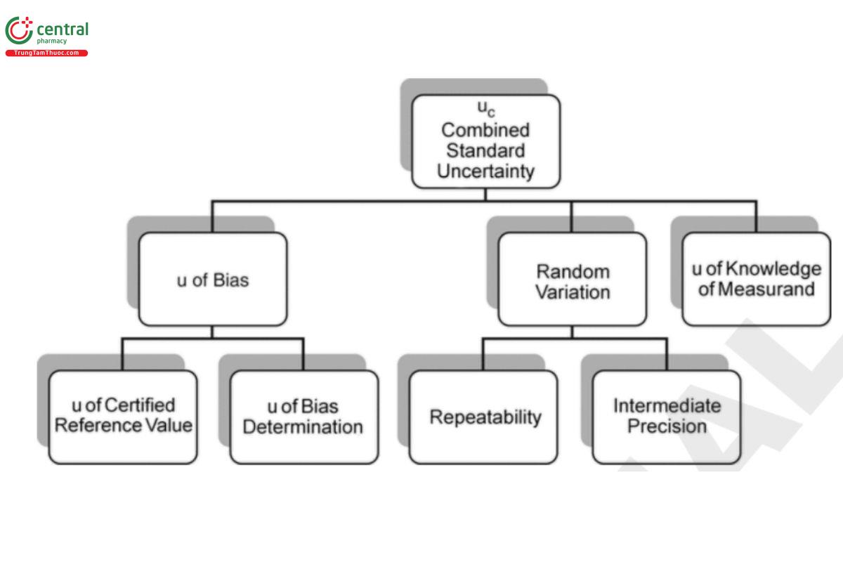
GUM notes the evaluation of measurement uncertainty is neither a routine task nor a purely mathematical one. Judgment is essential in choosing which uncertainty components (i.e., potential causes of measurement uncertainty) to consider in procedure development, qualification, and measurement uncertainty evaluation. For example, when preparing a 1 mg/L solution, the process by which it is prepared can influence the nal concentration. The analyst knows it would not be wise to weigh 1 mg of the substance followed by dilution to 1 L. Instead, recognizing the limits of typical analytical balances, a more precise result would be achieved by weighing 100 mg of substance and then serially diluting to the required concentration.

Measurement uncertainty arises from many sources including differences in instruments, mathematical algorithms, and analysts. A tutorial sampling of typical uncertainty components is provided in Table 12.

Table 12. A Tutorial List of Uncertainty Components in Analytical Laboratory Practice

A detailed discussion of measurement uncertainty in the pharmaceutical industry that expands upon the metrological principles introduced here and provides detailed definitions is provided in Weitzel et al. (27). In addition, a worked example for a drug substance is provided in Weitzel et al. (28).

10 APPENDIX 5: BAYESIAN INFERENCE

When describing statistical intervals in 3. Basic Statistical Principles and Uncertainty, it was noted that one can utilize a Bayesian approach to derive an interval which contains, with probability 100 × (1 − α)% the true value of the population mean. This is important because it returns a statement that the laboratory frequently wishes to make. This section will describe Bayesian inference and contrast it with frequentist inference which is more commonly understood throughout the pharmaceutical industry. Frequentist theory bases inferences on probability statements about statistics, while Bayesian inference is based on probability statements about population parameters. Population parameters are the unknowns that appear in statistical models (e.g., means, variances, difference of means) and statistics are summary measures or estimates based on data (e.g., parameter estimates). Frequentist inference regards parameter values as fixed and unknowable whereas Bayesian inference models their uncertainty using probability distributions. For instance the statement “there is a 95% probability that the difference in population means is between −0.1 to 0.1” is meaningless from a frequentist viewpoint, but reasonable from a Bayesian perspective. The Bayesian formulation offers a way for scientists needing to make risk based decisions. Bayesian inference can also incorporate prior information about statistical parameters together with the sample data to update what is known about a parameter. The ability to incorporate justified prior information potentially leads to better decisions when a study size is small, or when a factor is not adequately represented in the study design.

The purpose of this appendix is to provide a basic introduction to Bayesian inference applied to statistical studies and to analytical measurements. Gelman et al. (12) provides a source for more information.

10.1 Parameter Uncertainty versus Sampling Variability

Parameters are unknown hypothetical or population quantities, such as the mean or standard deviation of a population, or the difference in means between procedures. While unknown a parameter can be estimated. The estimation of a parameter and the inherent uncertainty of that estimation is the basis of Bayesian thinking.

Statistics are observed quantities or summaries of observed quantities in a sample taken from a population or process of interest. Examples of statistics include an analytical result (a measurement), a sample mean, a sample standard deviation, a difference in observed means between procedures, or their estimated confidence bounds. On repeated sampling of the population, the observed values of statistics will differ because of sampling variability.

Frequentist statistical methodology considers parameters to be fixed values that do not change. It employs probability theory to model the sampling variability of statistics randomly obtained from the population. These sampling distributions are then used to make inferences about the fixed value of the parameter. A common frequentist methodology is the calculation of a confidence interval. The process of computing a 95% confidence interval ensures that the realized interval will contain (or cover) the unknown parameter 95% of the time on repeated use.

The 95% refers to the reliability of the methodology (i.e., its coverage), and not the probability that the parameter falls within the interval. For example, suppose a computed 95% confidence interval on a mean is from 980 to 990 mg/g. It is not correct to state there is a 95% probability that the population mean is between 980 and 990 mg/g. To associate a probability with a fixed interval such as 980 to 990 mg/g, one must assume uncertainty is associated with the underlying parameter (i.e., it is not a fixed quantity). Rather, the 95% description of the

confidence interval means that the interval will correctly contain the true parameter value in 95% of repeated sampling applications from the population. The 95% refers to the success rate of the sampling process and not the parameter (which is assumed fixed). Bayesian statistical methodology considers a parameter value to be uncertain (not fixed), and models its likely levels using a probability distribution. It extends frequentist statistical methodology, using probability theory to model both the sampling variability of statistics and the decision maker’s uncertainty associated with parameters. Bayesian models are sometimes called “complete” probability models because they quantify the uncertainty associated with the parameters of interest, given the assumed sampling variability of the observed statistics, any relevant prior information, and the observed data. For instance, it is correct to say that a given Bayesian 95% credible interval (Bayesian analog of the confidence interval) contains the value of a specific parameter of interest with 95% probability (conditional on the observed data and other modeling assumptions). The same principles apply to the Bayesian analogs of frequentist tolerance and prediction intervals. Unlike frequentist interval methodology in which the probability level must be fixed in advance (e.g., 95%) and the resulting interval is random, Bayesian methodology offers the opportunity to x the interval in advance, and estimate the probability that the parameter value lies within that interval. Such an application is extremely useful for determining the probability that an analytical procedure will provide a signal outside a given range.

10.2 Prior and Posterior Distributions

Both frequentist and Bayesian methodologies express models using probability distributions. Both use the same model for sampling variability known as the likelihood. The particular likelihood model choice is based on prior knowledge concerning statistical variability. Bayesian inference also requires a probability model for parameter uncertainty, prior to observing the data, called the prior distribution. As with the likelihood, the prior distribution is a choice based on prior data, reliable knowledge, or common sense (e.g., the values of many parameters, such as a standard deviation, must be positive). Bayesian methodology requires care to assure that the chosen prior distributions are scientifically justified and do not unduly influence the inference. Use of appropriately justified knowledge of a prior distribution can potentially reduce sample size requirements for decision making. However, when there is little available theory, historical data, or expert knowledge available, prior distributions can be constructed that give minimal preference to any particular parameter value, and thus have minimal impact on the inference. Such prior distributions are often referred to as “non-informative”. When non-informative prior distributions are employed, inferences typically agree with the frequentist counterparts since both are solely dependent on the likelihood.

Bayesian methodology combines likelihood and prior distributional models with observed data to produce an updated distributional model for parameter uncertainty called the posterior distribution. The posterior distribution provides the probability that the population parameter value lies within any interval of interest. Such intervals are called credible intervals. When certain classes of non-informative prior distributions (e.g., a Jeffrey prior used with a normal likelihood) are employed, a Bayesian credible interval can be calculated from the posterior distribution, and may sometimes be numerically equal to the corresponding traditional confidence interval. However, as previously noted, the interpretations of these intervals are different. The probability associated with the credible interval quantifies uncertainty in an estimated parameter value conditional on observed data, while the probability associated with the confidence interval quantifies the probability of coverage of the estimated parameter on repeated estimation over many data sets.

From the Bayesian perspective, all knowledge about the parameter of interest is based on the posterior distribution. The posterior distribution from a previous study can inform the prior distribution for a subsequent study. Updating the prior distribution in this manner as new data become available, provides a paradigm for knowledge building, and thus a statistical basis for applying prior knowledge during pharmaceutical development (see ICH Q8(R2), Pharmaceutical Development [15]).

The posterior distribution of parameters may also be re-combined with the likelihood to obtain a posterior predictive distribution of future observed data or statistics. As with the posterior distribution, the Bayesian perspective bases all knowledge about future values on this posterior predictive distribution, which can be used to construct Bayesian analogs of frequentist tolerance and prediction intervals. Unlike the frequentist analogs, the Bayesian intervals do not require a prespecified fixed probability level. A posterior predictive distribution can be used, for example, in estimating the probability of occurrence of future out-of-specification results.

10.3 An Illustrative Example

Consider an analytical procedure for strength of drug product. The output of the procedure is a reportable value (mg/g) that estimates the mean strength, μ, for the tested lot of drug product. For the lot to be considered safe and effective, μ must be between 980 and 1020 mg/g. The observed reportable result, Y, is 1010 mg/g.

A typical rule used for disposition is to release the lot if 980 ≤ Y ≤ 1020. However, this rule is based on an observed reportable result that includes measurement error from the analytical procedure. What we really want to know is whether μ falls within the specification limits. This question can be informed using a Bayesian rule that releases the lot if the posterior probability that 980 ≤ μ ≤ 1020 is above some lower limit (e.g., 0.95). That is, we release the lot if the probability that the true value is within specifications is at least 0.95. Such a rule might be called a minimum posterior probability (MPP) rule. The MPP rule provides a probability based metric for acceptance of the lot under test.

The estimation of this posterior probability requires denifitions of the likelihood model and its parameters, the prior distributions of these parameters, and the data. For this illustration, the following are assumed:

- Likelihood: Reportable results follow a normal distribution with two unknown parameters: the population mean (μ) and intermediate precision standard deviation (σ). [Note—It is assumed the lot is homogeneous.]

- Prior distributions

Prior distribution of μ: There is no prior information on the strength of this lot. To represent this lack of knowledge assume a wide uniform distribution over the analytical range. The uniform distribution gives equal probability to any range of a given length regardless of location.

Prior distribution of σ: Data collected during validation resulted in an estimated intermediate precision variance (σ²_O) of 25 based on a sample of 10 independent reportable values. Based on this information, assume that σ² follows a scaled-inverse chi-squared distribution (a common prior distributional choice for variances) having df₀ = 10 − 1= 9 prior degrees of freedom and a prior scale parameter of σ_O = √25 = 5 mg/g.

- Data: A reportable value, Y = 1010 mg/g

Given the above information, the Bayes rule leads to a Student-t posterior distribution for (μ − Y)/σ_O with df_O = 9 degrees of freedom. The integration of this posterior distribution over the fixed range for μ of 980 to 1020 mg/g can be conveniently obtained using commonly available spreadsheet functions. For example, in Excel this is computed using the formulas, =T.DIST((1020–1010)/5,9,TRUE) − T.DIST((980– 1010)/5,9,TRUE). The resulting posterior probability that 980 ≤ μ ≤ 1020 for the tested lot is 0.96. That is, there is a 100 × 0.96 = 96% chance that the true mean of the lot falls within the specification limits. Because 0.96 > 0.95, the lot would be accepted based upon the MPP rule. The estimated posterior probability of 0.96 serves as a quantitative risk-based measure of the quality of the lot.

In this example, the parameter of interest is μ, a measurand quantity value. An analogous approach is used for Bayesian inference of other model parameters, such as the estimation of the difference in population means for two procedures, the underlying slope and intercept in a simple linear regression model, or performing tests of statistical equivalence.

In more complex situations (e.g., for complex, non-normal, or nonlinear models), Bayesian inference utilizes a form of computer simulation referred to as Markov-Chain Monte-Carlo (MCMC) simulation which is conducted using specialized software. MCMC technology requires care to assure that the MCMC iterations converge properly to the population posterior distribution.

10.4 A Comparison of Frequentist and Bayesian Methods

Both frequentist and Bayesian approaches to inference are useful. Frequentist approaches are widely available, straightforward, and offer the reliability of known coverage probability. Bayesian approaches can be used to quantify the uncertainty in parameters of interest which can support quantitative risk based decision making. While often more technically challenging to apply, Bayesian MCMC methodology can often be applied to problems that are intractable by frequentist approaches. When informative prior distributions can be justified, Bayesian methods may require smaller samples sizes for decision making than frequentist statistical methods. Table 13 provides a comparison of some characteristics from both frequentist and Bayesian perspectives.

Table 13. Characteristic Differences Between Frequentist and Bayesian Inference

11 REFERENCES

1. American Society for Testing Materials. Standard Practice for Using Significant Digits in Test Data to Determine Conformance with Specifications (ASTM E29–13). West Conshohocken, PA: ASTM International; 2013.

2. American Society for Testing Materials. Standard Practice for Dealing with Outlying Observations (ASTM E178–16a). West Conshohocken, PA: ASTM International; 2016.

3. American Society for Testing Materials. Standard Practice for Use of Control Charts in Statistical Process Control (ASTM E2587–16). West Conshohocken, PA: ASTM International; 2016.

4. Barnett KL, McGregor PL, Martin GP, LeBlond DJ, Weitzel MLJ, Ermer J, et al. Analytical target profile: structure and application throughout the analytical lifecycle. Pharm Forum. 2016;42(5).

5. Barnett V, Lewis T. Outliers in Statistical Data. 3rd ed. New York, NY: John Wiley and Sons; 1994.

6. Beckman RJ, Cook RD. Outlier … … … s. Technometrics. 1983; 25(2):119–149.

7. Böhrer A. One-sided and two-sided critical values for Dixon's Outlier Test for sample sizes up to n = 30. Economic Quality Control. 2008; 23(1):5–13.

8. Bristol DR. Probabilities and sample sizes for the two one-sided tests procedure. Communications in Statistics—Theory and Methods. 1993;22(7):1953–1961.

9. Chateld MJ, Borman PJ. Acceptance criteria for method equivalency assessments. Anal. Chem. 2009; 81(24):9841–9848. 10. Dixon WJ. Analysis of extreme values. Annals of Mathematical Statistics. 1950; 21(4):488–506.

11. Dixon WJ. Ratios involving extreme values. Annals of Mathematical Statistics. 1951; 22(1):68–78.

12. Gelman A, Carlin JB, Stern HS, Dunson DB, Vehtari A, Rubin DB. Bayesian Data Analysis. 3rd ed. Boca Raton, FL: Chapman & Hall/CRC Press; 2013.

13. Hauck WW, DeStefano AJ, Cecil TL, Abernethy DR, Koch WF, Williams RL. Acceptable, equivalent, or better: approaches for alternatives to oficial compendial procedures. Pharm Forum. 2010; 36(4):1077.

14. Hawkins DM. Identification of Outliers. New York: Chapman and Hall; 1980.

15. International Conference on Harmonization. Pharmaceutical Development: Q8(R2). Geneva Switzerland: ICH; 2009. https://database.ich.org/sites/default/les/Q8%28R2%29%20Guideline.pdf

16. Joint Committee for Guides in Metrology. Evaluation of Measurement Data—Guide to the Expression of Uncertainty in Measurement (GUM). Sèvres Cedex, France: Bureau International des Poids et Mesures; 2008.

17. Kirkwood TBL. Geometric means and measures of dispersion. Biometrics. 1979; 35(4):908–909.

18. Kringle R, Khan-Malek R, Snikeris F, Munden P, Agut C, Bauer M. A unified approach for design and analysis of transfer studies for analytical methods. Ther Infino Regul Sci. 2001; 35 (4):1271–1288.

19. Montgomery DC. Introduction to Statistical Quality Control. 7th ed., New York, NY: Wiley; 2012.

20. Nelson LS. Technical aids. Journal of Quality Technology. 1984; 16(4):238–239.

21. Oce of Regulatory Affairs. Laboratory Manual of Quality Policies. Vol. I of Laboratory Manual. 2017. www.fda.gov/science research/eld-science-and-laboratories/eld-science-laboratory-manual.

22. Oce of Regulatory Affairs. Laboratory Manual of Quality Policies. Vol. II of Laboratory Manual. 2017. www.fda.gov/science research/eld-science-and-laboratories/eld-science-laboratory-manual.

23. Oce of Regulatory Affairs. Laboratory Manual of Quality Policies. Vol. III, Sect 4.3 of Laboratory Manual. 2017. www.fda.gov/science research/eld-science-and-laboratories/eld-science-laboratory-manual.

24. National Institute of Standards and Technology. NIST/SEMATECH e-Handbook of Statistical Methods. 2012. http://www.itl.nist.gov/div898/handbook/.

25. Tan CY. RSD and other variability measures of the lognormal distribution. Pharm Forum. 2005; 31(2).

26. Torbeck LD, Statistical solutions: %RSD: friend or foe? Pharm Tech. 2010; 34(1):37–38.

27. Weitzel MLJ, Meija J, LeBlond D, Walsh S. Measurement uncertainty for the pharmaceutical industry. Pharm Forum. 2018; 44 (1). 2. Weitzel MLJ, LeBlond DJ, Burdick RK. Analytical quality by design approach to the development stage in the lifecycle of an analytical procedure. The Journal of Validation Technology. 2017; 23(5). www.ivtnetwork.com/article/analytical-quality-design-approach development-stage-lifecycle-analytical-procedure.

29. Wheeler DJ, Chambers DS. Understanding Statistical Process Control. 3rd ed. Knoxville, TN: SPC Press; 2012.